11.2: Voltaje relacionado con el campo

10.2.1 Una dimensión

El voltaje es energía eléctrica por unidad de carga, y el campo eléctrico es fuerza por unidad de carga. Para una partícula que se mueve en una dimensión, a lo largo del\(x\) eje, podemos relacionar voltaje y campo si partimos de la relación entre energía de interacción y fuerza,

\[\begin{equation*} dU = -F_xdx , \end{equation*}\]

y dividir por carga,

\[\begin{equation*} \frac{dU}{q} = -\frac{F_x}{q}dx , \end{equation*}\]

dando

\[\begin{equation*} dV = -E_x dx , \end{equation*}\]

o

\[\begin{equation*} \frac{dV}{dx} = -E_x . \end{equation*}\]

La interpretación es que un campo eléctrico fuerte ocurre en una región del espacio donde el voltaje está cambiando rápidamente. Por analogía, una ladera empinada es un lugar en el mapa donde la altitud está cambiando rápidamente.

Ejemplo 6: Campo generado por una anguila eléctrica

\(\triangleright\)Supongamos que una anguila eléctrica mide 1 m de largo, y genera una diferencia de voltaje de 1000 voltios entre su cabeza y cola. ¿Cuál es el campo eléctrico en el agua que lo rodea? \(\triangleright\)Sólo estamos calculando la cantidad de campo, no su dirección, por lo que ignoramos los signos positivos y negativos. Sujeto a la suposición posiblemente inexacta de un campo constante paralelo al cuerpo de la anguila, tenemos \[\begin{align*} |\mathbf{E}| &= \frac{dV}{d x} \\ &\approx \frac{\Delta V}{\Delta x} \text{[assumption of constant field]} \\ &= 1000\ \text{V/m} . \end{align*}\]

Ejemplo 7: Relacionar las unidades de campo eléctrico y voltaje

De nuestra definición original del campo eléctrico, esperamos que tenga unidades de newtons por culombo, N/C El ejemplo anterior, sin embargo, salió en voltios por metro, V/m. ¿Son estos inconsistentes? Tranquilémonos de que todo esto funciona. En este tipo de situaciones, la mejor estrategia suele ser simplificar las unidades más complejas para que solo involucren unidades mks y culombios. Dado que el voltaje se define como energía eléctrica por unidad de carga, tiene unidades de J/C: \[\begin{align*} \frac{\text{V}}{\text{m}} &= \frac{\text{J/C}}{\text{m}} \\ &= \frac{\text{J}}{\text{C}\cdot\text{m}} . \end{align*}\] Para conectar julios a newtons, recordamos que el trabajo es igual a fuerza por distancia, entonces\(\text{J}=\text{N}\cdot\text{m}\), entonces \[\begin{align*} \frac{\text{V}}{\text{m}} &= \frac{\text{N}\cdot\text{m}}{\text{C}\cdot\text{m}} \\ &= \frac{\text{N}}{\text{C}} \end{align*}\] Al igual que con otras dificultades de este tipo con las unidades eléctricas, uno comienza rápidamente a reconocer combinaciones que ocurren con frecuencia.

Ejemplo 8: Voltaje asociado a una carga puntual

\(\triangleright\)¿Cuál es el voltaje asociado a una carga puntual? \(\triangleright\)Como se derivó anteriormente en la autocomprobación A en la página 563, el campo es \[\begin{equation*} |\mathbf{E}| = \frac{ kQ}{ r^2} \end{equation*}\] La diferencia de voltaje entre dos puntos en la misma línea de radio es \[\begin{align*} \Delta V &= -\int d V \\ &= -\int E_{x} d x \end{align*}\] En la discusión general anterior,\(x\) era sólo un nombre genérico para la distancia recorrida a lo largo de la línea de un punto a otro, así que en este caso\(x\) realmente significa\(r\). \[\begin{align*} \Delta V &= -\int_{ r_1}^{ r_2} E_{r} d r \\ &= -\int_{ r_1}^{ r_2} \frac{ kQ}{ r^2} d r \\ &= \left.\frac{ kQ}{ r}\right]_{ r_1}^{ r_2} \ &= \frac{ kQ}{ r_2}-\frac{ kQ}{ r_1} . \end{align*}\] La convención estándar es usar\(r_1=\infty\) como punto de referencia, de manera que el voltaje a cualquier distancia\(r\) de la carga sea \[\begin{equation*} V = \frac{ kQ}{ r} . \end{equation*}\] La interpretación es que si acercas una carga de prueba positiva a una carga positiva, se incrementa su energía eléctrica; si fuera liberada, saltaría, liberando esta como energía cinética.

autocomprobación:

Demuestre que puede recuperar la expresión para el campo de una carga puntual evaluando la derivada\(E_{x}=-d V/d x\).

(respuesta en la parte posterior de la versión PDF del libro)

10.2.2 Dos o tres dimensiones

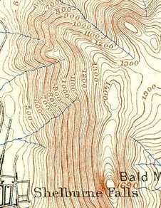
a / A topographical map of Shelburne Falls, Mass. (USGS).

The topographical map in figure a suggests a good way to visualize the relationship between field and voltage in two dimensions. Each contour on the map is a line of constant height; some of these are labeled with their elevations in units of feet. Height is related to gravitational energy, so in a gravitational analogy, we can think of height as representing voltage. Where the contour lines are far apart, as in the town, the slope is gentle. Lines close together indicate a steep slope.

If we walk along a straight line, say straight east from the town, then height (voltage) is a function of the east-west coordinate \(x\). Using the usual mathematical definition of the slope, and writing \(V\) for the height in order to remind us of the electrical analogy, the slope along such a line is \(dV/dx\) (the rise over the run).

What if everything isn't confined to a straight line? Water flows downhill. Notice how the streams on the map cut perpendicularly through the lines of constant height.

It is possible to map voltages in the same way, as shown in figure b. The electric field is strongest where the constant-voltage curves are closest together, and the electric field vectors always point perpendicular to the constant-voltage curves.

b / The constant-voltage curves surrounding a point charge. Near the charge, the curves are so closely spaced that they blend together on this drawing due to the finite width with which they were drawn. Some electric fields are shown as arrows.

The one-dimensional relationship \(E=-dV/dx\) generalizes to three dimensions as follows:

\[\begin{align*} E_x &= -\frac{dV}{dx} \\ E_y &= -\frac{dV}{dy} \\ E_z &= -\frac{dV}{dz} \end{align*}\]

This can be notated as a gradient (page 215),

\[\begin{equation*} \mathbf{E} = \nabla V , \end{equation*}\]

and if we know the field and want to find the voltage, we can use a line integral,

\[\begin{equation*} \Delta V = \int_C \mathbf{E}\cdot d\mathbf{r} , \end{equation*}\]

where the quantity inside the integral is a vector dot product.

self-check:

Imagine that figure a represents voltage rather than height. (a) Consider the stream the starts near the center of the map. Determine the positive and negative signs of \(dV/dx\) and \(dV/dy\), and relate these to the direction of the force that is pushing the current forward against the resistance of friction. (b) If you wanted to find a lot of electric charge on this map, where would you look?

(answer in the back of the PDF version of the book)

Figure c shows some examples of ways to visualize field and voltage patterns.

c / Two-dimensional field and voltage patterns. Top: A uniformly charged rod. Bottom: A dipole. In each case, the diagram on the left shows the field vectors and constant-voltage curves, while the one on the right shows the voltage (up-down coordinate) as a function of x and y. Interpreting the field diagrams: Each arrow represents the field at the point where its tail has been positioned. For clarity, some of the arrows in regions of very strong field strength are not shown --- they would be too long to show. Interpreting the constant-voltage curves: In regions of very strong fields, the curves are not shown because they would merge together to make solid black regions. Interpreting the perspective plots: Keep in mind that even though we're visualizing things in three dimensions, these are really two-dimensional voltage patterns being represented. The third (up-down) dimension represents voltage, not position.

Contributors

Template:ContribCrowell