3.5: La Integral Gaussiana

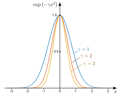
Aquí hay una integral famosa:\[\int_{-\infty}^\infty \; e^{-\gamma x^2} \; dx.\] El integrando se llama gaussiano, o curva de campana, y se traza a continuación. Cuanto mayor sea el valor de\(\gamma\), más estrecho alcanzó el pico de la curva.

Figura\(\PageIndex{1}\)

La integral fue resuelta por Gauss de una manera brillante. Dejar\(I(\gamma)\) denotar el valor de la integral. Entonces\(I^2\) son solo dos copias independientes de la integral, multiplicadas juntas:\[I^2(\gamma) = \left[\int_{-\infty}^\infty dx\; e^{-\gamma x^2}\right] \times \left[\int_{-\infty}^\infty dy\; e^{-\gamma y^2}\right].\] Tenga en cuenta que en la segunda copia de la integral, hemos cambiado la etiqueta “ficticio”\(x\) (la variable de integración) en\(y\), para evitar ambigüedades. Ahora, esto se convierte en una integral bidimensional, tomada sobre todo el plano 2D:\[I^2(\gamma) = \int_{-\infty}^\infty dx\, \int_{-\infty}^\infty dy \; e^{-\gamma (x^2+y^2)}.\] A continuación, cambiar de coordenadas cartesianas a polares:\[I^2(\gamma) = \int_{0}^\infty dr\, r \int_{0}^{2\pi} d\phi \; e^{-\gamma r^2} = \left[ \int_{0}^\infty dr\, r \, e^{-\gamma r^2}\right] \times \left[\int_{0}^{2\pi} d\phi \right] = \frac{1}{2\gamma} \cdot 2\pi.\] Al tomar la raíz cuadrada, llegamos al resultado\[I(\gamma) = \int_{-\infty}^\infty dx \; e^{-\gamma x^2} = \sqrt{\frac{\pi}{\gamma}}.\]