10A: Problemas de aceleración constante en dos dimensiones

Al resolver problemas que implican aceleración constante en dos dimensiones, el error más común es probablemente mezclar el\(x\) and \(y\) motion. One should do an analysis of the \(x\) motion and a separate analysis of the \(y\) motion. The only variable common to both the \(x\) and the \(y\) motion is the time. Note that if the initial velocity is in a direction that is along neither axis, one must first break up the initial velocity into its components.

En los últimos capítulos hemos considerado el movimiento de una partícula que se mueve a lo largo de una línea recta con aceleración constante. En tal caso, la velocidad y la aceleración siempre se dirigen a lo largo de una misma línea, la línea sobre la que se mueve la partícula. Aquí seguimos restringiéndonos a casos que implican aceleración constante (constante tanto en magnitud como en dirección) pero levantamos la restricción de que la velocidad y la aceleración sean dirigidas a lo largo de una misma línea. Si la velocidad de la partícula en el tiempo cero no es colineal con la aceleración, entonces la velocidad nunca será colineal con la aceleración y la partícula se moverá a lo largo de una trayectoria curva. La trayectoria curva se limitará al plano que contiene tanto el vector de velocidad inicial como el vector de aceleración, y en ese plano, la trayectoria será una parábola. (La trayectoria es solo el camino de la partícula.)

Vas a ser responsable de lidiar con dos clases de problemas que implican aceleración constante en dos dimensiones:

1. Problemas que implican el movimiento de una sola partícula.
2. Problemas de colisión tipo II en dos dimensiones

Utilizamos problemas de muestra para ilustrar los conceptos que debes entender para resolver problemas bidimensionales de aceleración constante.

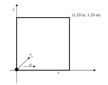
Un cuadrado horizontal de longitud de borde\(1.20\) m is situated on a Cartesian coordinate system such that one corner of the square is at the origin and the corner opposite that corner is at (\(1.20\) m, \(1.20\) m). A particle is at the origin. The particle has an initial velocity of \(2.20\) m/s directed toward the corner of the square at (\(1.20\) m, \(1.20\) m) and has a constant acceleration of \(4.87 m/s^2\) in the \(+x\) direction. Where does the particle hit the perimeter of the square?

Solution

Let’s start with a diagram.

Now let’s make some conceptual observations on the motion of the particle. Recall that the square is horizontal so we are looking down on it from above. It is clear that the particle hits the right side of the square because: It starts out with a velocity directed toward the far right corner. That initial velocity has an \(x\) component and a \(y\) component. The \(y\) component never changes because there is no acceleration in the \(y\) direction. The \(x\) component, however, continually increases. The particle is going rightward faster and faster. Thus, it will take less time to get to the right side of the square then it would without the acceleration and the particle will get to the right side of the square before it has time to get to the far side.

An important aside on the trajectory (path) of the particle: Consider an ordinary checker on a huge square checkerboard with squares of ordinary size (just a lot more of them then you find on a standard checkerboard). Suppose you start with the checker on the extreme left square of the end of the board nearest you (square 1) and every second, you move the checker right one square and forward one square. This would correspond to the checker moving toward the far right corner at constant velocity. Indeed you would be moving the checker along the diagonal. Now let’s throw in some acceleration. Return the checker to square 1 and start moving it again. This time, each time you move the checker forward, you move it rightward one more square than you did on the previous move. So first you move it forward one square and rightward one square. Then you move it forward another square but rightward two more squares. Then forward one square and rightward three squares. And so on. With each passing second, the rightward move gets bigger. (That’s what we mean when we say the rightward velocity is continually increasing.) So what would the path of the checker look like? Let’s draw a picture.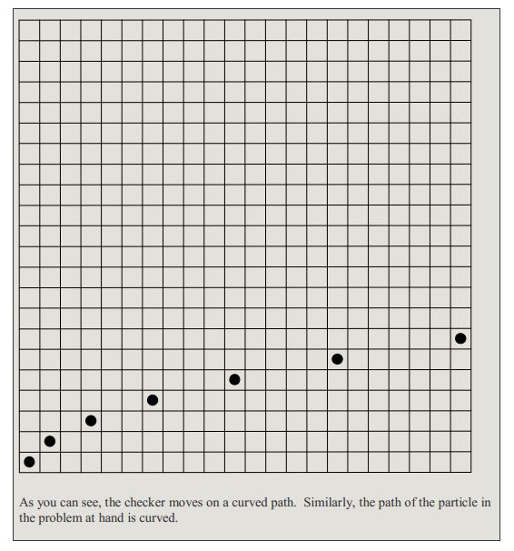

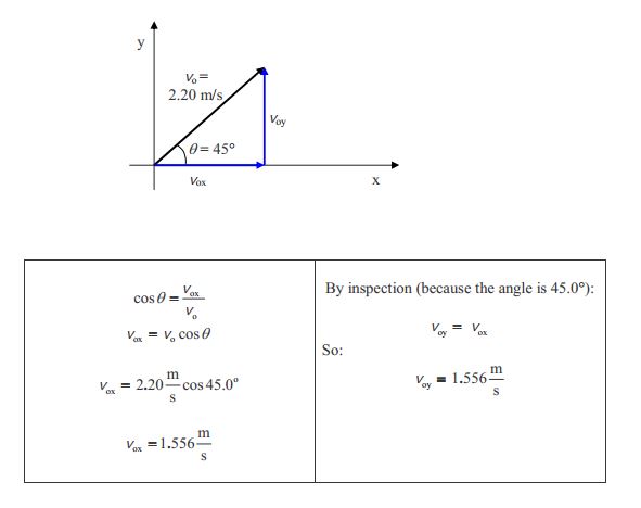
Ahora volvamos al problema que nos ocupa. La forma de atacar estos problemas bidimensionales de aceleración constante es tratar el\(x\) movimiento y el\(y\) movimiento por separado. La dificultad con eso, en el caso que nos ocupa, es que la velocidad inicial no es\(x\) ni a lo largo ni a lo largo\(y\) sino que de hecho es una mezcla tanto de\(x\) movimiento como de\(y\) movimiento. Lo que tenemos que hacer es separarlo en su\(x\) y\(y\) componentes. Vamos a proceder con eso. Tenga en cuenta que, por inspección, el ángulo que el vector de velocidad hace con el\(x\) eje es\(45.0^{\circ}\).

Ahora estamos listos para atacar el movimiento x y el movimiento y por separado. Antes de hacerlo, consideremos nuestro plan de ataque. Hemos establecido, por medio del razonamiento conceptual, que la partícula golpeará el lado derecho del cuadrado. Esto quiere decir que ya tenemos la respuesta a la mitad de la pregunta “¿Dónde golpea la partícula el perímetro de la plaza?” Le pega a\(x=1.20 m\) e y =? . Todo lo que tenemos que hacer es averiguar el valor de\(y\). Hemos establecido que es el\(x\) movimiento el que determina el tiempo que tarda la partícula en impactar el perímetro de la plaza. Golpea el perímetro de la plaza en ese instante en el tiempo cuando\(x\) logra el valor de\(1.20 m\). Entonces nuestro plan de ataque es usar una o más de las ecuaciones de aceleración constante\(x\) -motion para determinar el momento en el que la partícula golpea el perímetro del cuadrado y para tapar ese tiempo en la ecuación apropiada de aceleración constante de\(y\) movimiento para obtener el valor de\(y\) al cual la partícula golpea el lado del cuadrado. Vamos a por ello.

x movimiento
Comenzamos con la ecuación que relaciona posición y tiempo:

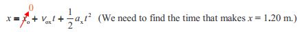
El\(x\) componente de la aceleración es la aceleración total, es decir\(a_x=a\). Por lo tanto,

\[x=v_{0x}t+\dfrac{1}{2}at^2\]

Reconociendo que estamos tratando con una ecuación cuadrática la obtenemos en la forma estándar de la ecuación cuadrática.

\[\dfrac{1}{2}at^2+v_{0x}t-x=0\]

Ahora aplicamos la fórmula cuadrática:

\[t=\dfrac{-v_{0x}\pm\sqrt{v_{0x}^2-4(\dfrac{1}{2}a)(-x)}}{2(\dfrac{1}{2}a_x)}\]

\[t=\dfrac{-v_{0x}\pm\sqrt{v_{0x}^2+2ax}}{a_x}\]

sustituyendo valores por unidades (y, en este paso, no haciendo evaluación) obtenemos:

\[t=\dfrac{-1.556\dfrac{m}{s}\pm\sqrt{(1.556\dfrac{m}{s})^2+2(4.87\dfrac{m}{s^2})1.20m}}{4.87\dfrac{m}{s^2}}\]

Al evaluar esta expresión se obtienen:

\[t=0.4518 s\]

y

\[t=−1.091 s.\]

Estamos resolviendo para un tiempo futuro así que eliminamos el resultado negativo con el argumento de que es un tiempo en el pasado. Hemos encontrado que la partícula llega al lado derecho de la plaza en el momento\(t=0.4518 s\). Ahora la pregunta es: “¿Cuál es el valor de\(y\) en ese momento?”

y movimiento

Nuevamente volvemos a la ecuación de aceleración constante que relaciona la posición con el tiempo, esta vez escribiéndola en términos de las\(y\) variables:

Observamos que\(y_0\) es cero porque la partícula está en el origen en el momento\(0\) y ay es cero porque la aceleración está en la\(+x\) dirección lo que significa que no tiene componente y. Reescribiendo esto:

\[y=V_{0y}t\]

Sustituir valores por unidades,

\[y=1.556\dfrac{m}{s}(0.4518s)\]

evaluar y redondear a tres cifras significativas rendimientos:

\[y=0.703m\]

Así, la partícula golpea el perímetro del cuadrado en

\[(1.20m,0.703m)\]

A continuación, consideremos un problema de colisión 2-D Tipo II. Resolver un problema típico de Colisión 2-D Tipo II implica encontrar la trayectoria de una de las partículas, encontrar cuándo la otra partícula cruza esa trayectoria y establecer dónde está la primera partícula cuando la segunda partícula cruza esa trayectoria. Si la primera partícula está en el punto de su propia trayectoria donde la segunda partícula cruza esa trayectoria entonces hay una colisión. En el caso de objetos en lugar de partículas, a menudo se tiene que hacer algún razonamiento adicional para resolver un problema de Colisión 2-D Tipo II. Tal razonamiento se ilustra en el siguiente ejemplo que involucra un cohete.

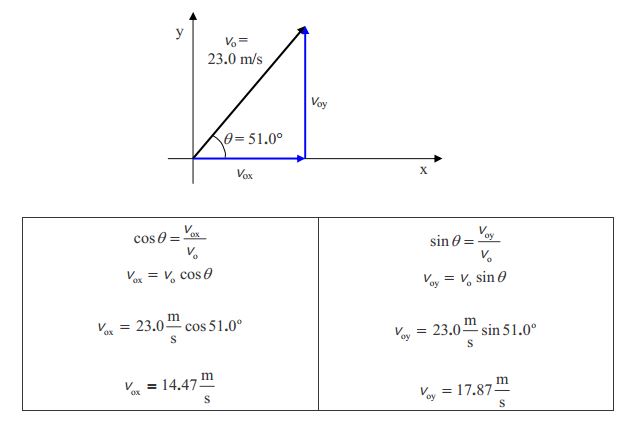
Las posiciones de una partícula y un cohete delgado (tratarlo como tan delgado como una línea) de longitud\(0.280 m\) are specified by means of Cartesian coordinates. At time \(0\) the particle is at the origin and is moving on a horizontal surface at \(23.0 m/s\) at \(51.0^\circ\). It has a constant acceleration of \(2.43 m/s^2\) in the \(+y\) direction. At time \(0\) the rocket is at rest and it extends from (\(−.280 m\), \(50.0 m\)) to (\(0\), \(50.0 m\)), but it has a constant acceleration in the \(+x\) direction. What must the acceleration of the rocket be in order for the particle to hit the rocket?

Solution

Based on the description of the motion, the rocket travels on the horizontal surface along the line \(y=50.0 m\). Let’s figure out where and when the particle crosses this line. Then we’ll calculate the acceleration that the rocket must have in order for the nose of the rocket to be at that point at that time and repeat for the tail of the rocket. Finally, we’ll quote our answer as being any acceleration in between those two values.

When and where does the particle cross the line \(y=50.0 m\)?

We need to treat the particle’s \(x\) motion and the \(y\) motion separately. Let’s start by breaking up the initial velocity of the particle into its \(x\) and \(y\) components.

Now in this case, it is the y motion that determines when the particle crosses the trajectory of the rocket because it does so when \(y=50.0 m\). So let’s address the y motion first.

y motion of the particle

Note that we can’t just assume that we can cross out yo but in this case the time zero position of the particle was given as (\(0\), \(0\)) meaning that \(y_o\) is indeed zero for the case at hand. Now we solve for \(t\):

\[y=V_{0y}t+\dfrac{1}{2}a_yt^2\]

\[\dfrac{1}{2}a_yt^2+V_{0y}t-y=0\]

\[t=\dfrac{-V_{0y}\pm\sqrt{V_{0y}^2-4(\dfrac{1}{2}a_y)(-y)}}{2(\dfrac{1}{2}a_y)}\]

\[t=\dfrac{-V_{0y}\pm\sqrt{V_{0y}^2+2a_yy}}{a_y}\]

\[t=\dfrac{-17.87\dfrac{m}{s}\pm\sqrt{(17.87\dfrac{m}{s})^2+2(2.43\dfrac{m}{s^2})50.0m}}{2.43\dfrac{m}{s^2}}\]

\(t=2.405s\) and \(t=-17.11s\)

Again, we throw out the negative solution because it represents an instant in the past and we want a future instant. Now we turn to the x motion to determine where the particle crosses the trajectory of the rocket.

x motion of the particle
Again we turn to the constant acceleration equation relating position to time, this time writing it in terms of the x variables:

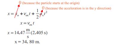
So the particle crosses the rocket’s path at (\(34.80 m\), \(50.0 m\)) at time \(t=2.450 s\). Let’s calculate the acceleration that the rocket would have to have in order for the nose of the rocket to be there at that instant. The rocket has \(x\) motion only. It is always on the line \(y = 50.0 m\).

Motion of the Nose of the Rocket

where we use the subscript n for “nose” and a prime to indicate “rocket.” We have crossed out \(x'_{on}\) because the nose of the rocket is at (\(0\), \(50.0 m\)) at time zero, and we have crossed out \(v'_{oxn}\) because the rocket is at rest at time zero.

\[x'_n=\dfrac{1}{2}a'_nt^2\]

Solving for \(a'_n\) yields:

\[a'_n=\dfrac{2x'_n}{t^2}\]

Now we just have to evaluate this expression at \(t = 2.405 s\), the instant when the particle crosses the trajectory of the rocket, and at \(x'_n=x= 34.80 m\), the value of \(x\) at which the particle crosses the trajectory of the rocket.

\[a'_n=\dfrac{2(34.80m)}{(2.405s)^2}\]

\[a'_n=12.0\dfrac{m}{s^2}\]

It should be emphasized that the \(n\) for “nose” is not there to imply that the nose of the rocket has a different acceleration than the tail; rather; the whole rocket must have the acceleration \(a′_n=12.0\dfrac{m}{s^2}\) in order for the particle to hit the rocket in the nose. Now let’s find the acceleration at′that the entire rocket must have in order for the particle to hit the rocket in the tail.

Motion of the Tail of the Rocket

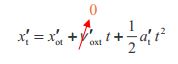
where we use the subscript \(t\) for “tail” and a prime to indicate “rocket.” We have crossed out \(v′_{oxt}\) because the rocket is at rest at time zero, but \(x'_{ot}\) is not zero because the tail of the rocket is at (\(−.280\), \(50.0 m\)) at time zero.

\[x'_t=x'_{ot}+\dfrac{1}{2}a'_tt^2\]

Solving for \(a'_t\) yields:

\[a'_t=\dfrac{2(x'_t-x'_{ot})}{t^2}\]

Evaluating at \(t = 2.405 s\) and \(x'_t= x = 34.80 m\) yields

\[a'_t=\dfrac{2(34.80m-(-0.280m))}{(2.405s)^2}\]

\[a'_t=12.1\dfrac{m}{s^2}\]

as the acceleration that the rocket must have in order for the particle to hit the tail of the rocket.

Thus: The acceleration of the rocket must be somewhere between \(12.0\dfrac{m}{s^2}\) and \(12.1\dfrac{m}{s^2}\), inclusive, in order for the rocket to be hit by the particle.