Search

Text Color

Margin Size

Font Type

Enable Dyslexic Font

9A: Gráficas de Movimiento Unidimensionales

Última actualización

30 oct 2022
Guardar como PDF
- 8A: Movimiento unidimensional: Colisión Tipo II
- 10A: Problemas de aceleración constante en dos dimensiones

$\newcommand{\vecs}[1]{\overset { \scriptstyle \rightharpoonup} {\mathbf{#1}} }$

$\newcommand{\vecd}[1]{\overset{-\!-\!\rightharpoonup}{\vphantom{a}\smash {#1}}}$

$\newcommand{\id}{\mathrm{id}}$ $\newcommand{\Span}{\mathrm{span}}$

( \newcommand{\kernel}{\mathrm{null}\,}\) $\newcommand{\range}{\mathrm{range}\,}$

$\newcommand{\RealPart}{\mathrm{Re}}$ $\newcommand{\ImaginaryPart}{\mathrm{Im}}$

$\newcommand{\Argument}{\mathrm{Arg}}$ $\newcommand{\norm}[1]{\| #1 \|}$

$\newcommand{\inner}[2]{\langle #1, #2 \rangle}$

$\newcommand{\Span}{\mathrm{span}}$

$\newcommand{\id}{\mathrm{id}}$

$\newcommand{\Span}{\mathrm{span}}$

$\newcommand{\kernel}{\mathrm{null}\,}$

$\newcommand{\range}{\mathrm{range}\,}$

$\newcommand{\RealPart}{\mathrm{Re}}$

$\newcommand{\ImaginaryPart}{\mathrm{Im}}$

$\newcommand{\Argument}{\mathrm{Arg}}$

$\newcommand{\norm}[1]{\| #1 \|}$

$\newcommand{\inner}[2]{\langle #1, #2 \rangle}$

$\newcommand{\Span}{\mathrm{span}}$ $\newcommand{\AA}{\unicode[.8,0]{x212B}}$

$\newcommand{\vectorA}[1]{\vec{#1}} % arrow$

$\newcommand{\vectorAt}[1]{\vec{\text{#1}}} % arrow$

$\newcommand{\vectorB}[1]{\overset { \scriptstyle \rightharpoonup} {\mathbf{#1}} }$

$\newcommand{\vectorC}[1]{\textbf{#1}}$

$\newcommand{\vectorD}[1]{\overrightarrow{#1}}$

$\newcommand{\vectorDt}[1]{\overrightarrow{\text{#1}}}$

$\newcommand{\vectE}[1]{\overset{-\!-\!\rightharpoonup}{\vphantom{a}\smash{\mathbf {#1}}}}$

$\newcommand{\vecs}[1]{\overset { \scriptstyle \rightharpoonup} {\mathbf{#1}} }$

$\newcommand{\vecd}[1]{\overset{-\!-\!\rightharpoonup}{\vphantom{a}\smash {#1}}}$

$\newcommand{\avec}{\mathbf a}$

$\newcommand{\bvec}{\mathbf b}$

$\newcommand{\cvec}{\mathbf c}$

$\newcommand{\dvec}{\mathbf d}$

$\newcommand{\dtil}{\widetilde{\mathbf d}}$

$\newcommand{\evec}{\mathbf e}$

$\newcommand{\fvec}{\mathbf f}$

$\newcommand{\nvec}{\mathbf n}$

$\newcommand{\pvec}{\mathbf p}$

$\newcommand{\qvec}{\mathbf q}$

$\newcommand{\svec}{\mathbf s}$

$\newcommand{\tvec}{\mathbf t}$

$\newcommand{\uvec}{\mathbf u}$

$\newcommand{\vvec}{\mathbf v}$

$\newcommand{\wvec}{\mathbf w}$

$\newcommand{\xvec}{\mathbf x}$

$\newcommand{\yvec}{\mathbf y}$

$\newcommand{\zvec}{\mathbf z}$

$\newcommand{\rvec}{\mathbf r}$

$\newcommand{\mvec}{\mathbf m}$

$\newcommand{\zerovec}{\mathbf 0}$

$\newcommand{\onevec}{\mathbf 1}$

$\newcommand{\real}{\mathbb R}$

$\newcommand{\twovec}[2]{\left[\begin{array}{r}#1 \\ #2 \end{array}\right]}$

$\newcommand{\ctwovec}[2]{\left[\begin{array}{c}#1 \\ #2 \end{array}\right]}$

$\newcommand{\threevec}[3]{\left[\begin{array}{r}#1 \\ #2 \\ #3 \end{array}\right]}$

$\newcommand{\cthreevec}[3]{\left[\begin{array}{c}#1 \\ #2 \\ #3 \end{array}\right]}$

$\newcommand{\fourvec}[4]{\left[\begin{array}{r}#1 \\ #2 \\ #3 \\ #4 \end{array}\right]}$

$\newcommand{\cfourvec}[4]{\left[\begin{array}{c}#1 \\ #2 \\ #3 \\ #4 \end{array}\right]}$

$\newcommand{\fivevec}[5]{\left[\begin{array}{r}#1 \\ #2 \\ #3 \\ #4 \\ #5 \\ \end{array}\right]}$

$\newcommand{\cfivevec}[5]{\left[\begin{array}{c}#1 \\ #2 \\ #3 \\ #4 \\ #5 \\ \end{array}\right]}$

$\newcommand{\mattwo}[4]{\left[\begin{array}{rr}#1 \amp #2 \\ #3 \amp #4 \\ \end{array}\right]}$

$\newcommand{\laspan}[1]{\text{Span}\{#1\}}$

$\newcommand{\bcal}{\cal B}$

$\newcommand{\ccal}{\cal C}$

$\newcommand{\scal}{\cal S}$

$\newcommand{\wcal}{\cal W}$

$\newcommand{\ecal}{\cal E}$

$\newcommand{\coords}[2]{\left\{#1\right\}_{#2}}$

$\newcommand{\gray}[1]{\color{gray}{#1}}$

$\newcommand{\lgray}[1]{\color{lightgray}{#1}}$

$\newcommand{\rank}{\operatorname{rank}}$

$\newcommand{\row}{\text{Row}}$

$\newcommand{\col}{\text{Col}}$

$\renewcommand{\row}{\text{Row}}$

$\newcommand{\nul}{\text{Nul}}$

$\newcommand{\var}{\text{Var}}$

$\newcommand{\corr}{\text{corr}}$

$\newcommand{\len}[1]{\left|#1\right|}$

$\newcommand{\bbar}{\overline{\bvec}}$

$\newcommand{\bhat}{\widehat{\bvec}}$

$\newcommand{\bperp}{\bvec^\perp}$

$\newcommand{\xhat}{\widehat{\xvec}}$

$\newcommand{\vhat}{\widehat{\vvec}}$

$\newcommand{\uhat}{\widehat{\uvec}}$

$\newcommand{\what}{\widehat{\wvec}}$

$\newcommand{\Sighat}{\widehat{\Sigma}}$

$\newcommand{\lt}{<}$

$\newcommand{\gt}{>}$

$\newcommand{\amp}{&}$

$\definecolor{fillinmathshade}{gray}{0.9}$

Considere un objeto que experimenta movimiento a lo largo de una trayectoria en línea recta, donde el movimiento se caracteriza por unos pocos intervalos de tiempo consecutivos durante cada uno de los cuales la aceleración es constante pero típicamente a un valor constante diferente al que es para los intervalos de tiempo especificados adyacentes. La aceleración experimenta cambios bruscos de valor al final de cada intervalo de tiempo especificado. El cambio abrupto conduce a una discontinuidad de salto en la Gráfica de Aceleración vs Tiempo y una discontinuidad en la pendiente (pero no en el valor) de la Gráfica de Velocidad vs Tiempo (así, hay una “esquina” o un “kink” en la traza de la gráfica Velocidad vs Tiempo). El caso es que la traza de la gráfica Posición vs Tiempo se extiende suavemente a través de esos instantes de tiempo en los que cambia la aceleración. Incluso las personas que se vuelven bastante competentes en la generación de las gráficas tienen una tendencia a incluir erróneamente una curva en la gráfica Posición vs Tiempo en un punto de la gráfica correspondiente a un instante en el que la aceleración sufre un cambio abrupto.

Tus metas aquí todas pertenecen al movimiento de un objeto que se mueve a lo largo de una trayectoria en línea recta a una aceleración constante durante cada uno de varios intervalos de tiempo pero con un cambio abrupto en el valor de la aceleración al final de cada intervalo de tiempo (excepto el último) al nuevo valor de aceleración que pertenece al siguiente intervalo de tiempo. Sus metas para tal movimiento son:

Dada una descripción (en palabras) del movimiento del objeto; producir una gráfica de posición vs tiempo, una gráfica de velocidad vs. tiempo, y una gráfica de aceleración vs. tiempo, para ese movimiento.
Dado un gráfico de velocidad vs tiempo, y la posición inicial del objeto; producir una descripción del movimiento, producir una gráfica de posición vs tiempo, y producir una gráfica de aceleración vs tiempo.
Dada una gráfica de aceleración vs. tiempo, la posición inicial del objeto y la velocidad inicial del objeto; producir una descripción del movimiento, producir una gráfica de posición vs tiempo y producir una gráfica de velocidad vs tiempo.

Se proporciona el siguiente ejemplo para comunicar más claramente lo que se espera de ti y lo que tienes que hacer para cumplir con esas expectativas:

Un automóvil se mueve por un tramo recto de carretera sobre el que se ha pintado una línea de salida. Al inicio de las observaciones, el auto ya está $225 m$ ahead of the start line and is moving forward at a steady $15 m/s$ . The car continues to move forward at $15 m/s$ for $5.0$ seconds. Then it begins to speed up. It speeds up steadily, obtaining a speed of $35 m/s$ after another $5.0$ seconds. As soon as its speed gets up to $35 m/s$ , the car begins to slow down. It slows steadily, coming to rest after another $10.0$ seconds. Sketch the graphs of position vs. time, velocity vs. time, and acceleration vs. time pertaining to the motion of the car during the period of time addressed in the description of the motion. Label the key values on your graphs of velocity vs. time and acceleration vs. time.

Solution

Okay, we are asked to draw three graphs, each of which has the time, the same “stopwatch readings” plotted along the horizontal axis. The first thing I do is to ask myself whether the plotted lines/curves are going to extend both above and below the time axis. This helps to determine how long to draw the axes. Reading the description of motion in the case at hand, it is evident that:

The car goes forward of the start line but it never goes behind the start line. So, the $x$ vs. $t$ graph will extend above the time axis (positive values of $x$ ) but not below it (negative values of $x$ ).

The car does take on positive values of velocity, but it never backs up, that is, it never takes on negative values of velocity. So, the $v$ vs. $t$ graph will extend above the time axis but not below it.

The car speeds up while it is moving forward (positive acceleration), and it slows down while it is moving forward (negative acceleration). So, the $a$ vs. $t$ graph will extend both above and below the time axis.

Next, I draw the axes, first for $x$ vs. $t$ , then directly below that set of axes, the axes for $v$ vs. $t$ , and finally, directly below that, the axes for $a$ vs. $t$ . Then I label the axes, both with the symbol used to represent the physical quantity being plotted along the axis and, in brackets, the units for that quantity.

Now I need to put some tick marks on the time axis. To do so, I have to go back to the question to find the relevant time intervals. I’ve already read the question twice and I’m getting tired of reading it over and over again. This time I’ll take some notes:

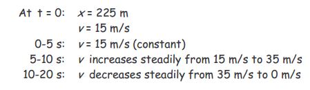
From my notes it is evident that the times run from $0$ to $20$ seconds and that labeling every $5$ seconds would be convenient. So I put four tick marks on the time axis of $x$ vs. $t$ . I label the origin $0$ , $0$ and label the tick marks on the time axis $5$ , $10$ , $15$ , and $20$ respectively. Then I draw vertical dotted lines, extending my time axis tick marks up and down the page through all the graphs. They all share the same times and this helps me ensure that the graphs relate properly to each other. In the following diagram we have the axes and the graph. Except for the labeling of key values I have described my work in a series of notes. To follow my work, please read the numbered notes, in order, from $1$ to $10$ .

alt

Los valores clave en el $v$ vs. $t$ gráfico son dados así que el único “misterio”, sobre el diagrama anterior, que queda es, “¿Cómo fueron los valores clave en $a$ vs $t$ obtenidos?” Aquí están las respuestas:

En el intervalo de tiempo de $t=5$ segundos a $t=10$ segundos, la velocidad cambia de $15\dfrac{m}{s}$ a $35\dfrac{m}{s}$ . Así, en ese intervalo de tiempo la aceleración viene dada por:

$a=\dfrac{\triangle v}{\triangle t}=\dfrac{v_f-v_i}{t_f-t_i}=\dfrac{35\dfrac{m}{s}-15\dfrac{m}{s}}{10s-5s}=4\dfrac{m}{s^2}$

En el intervalo de tiempo de $t=10$ segundos a $t=20$ segundos, la velocidad cambia de $35\dfrac{m}{s}$ a $0\dfrac{m}{s}$ . Así, en ese intervalo de tiempo la aceleración viene dada por:

$a=\dfrac{\triangle v}{\triangle t}=\dfrac{v_f-v_i}{t_f-t_i}=\dfrac{0\dfrac{m}{s}-35\dfrac{m}{s}}{20s-10s}=-3.5\dfrac{m}{s^2}$

Support Center

How can we help?