19.6: Momentum Angular de un Sistema de Partículas

Ahora calculamos el momento angular alrededor del punto\(S\) asociado a un sistema de partículas de N puntos. Marcar cada partícula individual por el índice\(j, j=1,2, \cdots, N\). Deja que la\(j^{\mathrm{th}}\) partícula tenga masa\(m_{j}\) y velocidad\(\overrightarrow{\mathbf{V}}\). El impulso de una partícula individual es entonces\(\overrightarrow{\mathbf{p}}_{j}=m_{j} \overrightarrow{\mathbf{v}}_{j}\). Dejar\(\overrightarrow{\mathbf{r}}_{S, j}\) ser el vector desde el punto\(S\) a la\(j^{\mathrm{th}}\) partícula, y dejar\(\theta_{j}\) ser el ángulo entre los vectores\(\overrightarrow{\mathbf{r}}_{S, j}\) y\(\overrightarrow{\mathbf{p}}_{j}\) (Figura 19.10).

Figura\(\PageIndex{1}\): Sistema de partículas

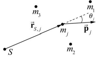
El momento angular\(\overrightarrow{\mathbf{L}}_{S, j}\) de la\(j^{\text {th }}\) partícula es

\[\overrightarrow{\mathbf{L}}_{S, j}=\overrightarrow{\mathbf{r}}_{S, j} \times \overrightarrow{\mathbf{p}}_{j} \nonumber \]

El momento angular para el sistema de partículas es la suma vectorial del momento angular individual,

\[\overrightarrow{\mathbf{L}}_{S}^{\mathrm{sys}}=\sum_{j=1}^{i=N} \overrightarrow{\mathbf{L}}_{S, j}=\sum_{j=1}^{i=N} \overrightarrow{\mathbf{r}}_{S, j} \times \overrightarrow{\mathbf{p}}_{j} \nonumber \]

El cambio en el momento angular del sistema de partículas alrededor de un punto\(S\) viene dado por

\[\frac{d \overrightarrow{\mathbf{L}}_{S}^{\mathrm{sys}}}{d t}=\frac{d}{d t} \sum_{j=1}^{j=N} \overrightarrow{\mathbf{L}}_{S, j}=\sum_{j=1}^{j=N}\left(\frac{d \overrightarrow{\mathbf{r}}_{S, j}}{d t} \times \overrightarrow{\mathbf{p}}_{j}+\overrightarrow{\mathbf{r}}_{S, j} \times \frac{d \overrightarrow{\mathbf{p}}_{j}}{d t}\right) \nonumber \]

Debido a que la velocidad de la\(j^{\text {th }}\) partícula es\(\overrightarrow{\mathbf{v}}_{S, j}=d{\mathbf{r}}_{S, j} / d t\), el primer término entre paréntesis se desvanece (el producto cruzado de un vector consigo mismo es cero porque son paralelos entre sí)

\[\frac{d \overrightarrow{\mathbf{r}}_{S, j}}{d t} \times \overrightarrow{\mathbf{p}}_{j}=\overrightarrow{\mathbf{v}}_{S, j} \times m_{j} \overrightarrow{\mathbf{v}}_{S, j}=0 \nonumber \]

Ecuación sustituta (19.5.4) y\(\overrightarrow{\mathbf{F}}_{j}=d \overrightarrow{\mathbf{p}}_{j} / d t\) en la ecuación (19.5.3) rendimiento

\[\frac{d \overrightarrow{\mathbf{L}}_{S}^{\mathrm{sys}}}{d t}=\sum_{j=1}^{i=N}\left(\overrightarrow{\mathbf{r}}_{S, j} \times \frac{d \overrightarrow{\mathbf{p}}_{j}}{d t}\right)=\sum_{j=1}^{i=N}\left(\overrightarrow{\mathbf{r}}_{S, j} \times \overrightarrow{\mathbf{F}}_{j}\right) \nonumber \]

Porque

\[\sum_{j=1}^{j=N}\left(\overrightarrow{\mathbf{r}}_{S, j} \times \overrightarrow{\mathbf{F}}_{j}\right)=\sum_{j=1}^{j=N} \vec{\tau}_{S, j}=\vec{\tau}_{S}^{\mathrm{ext}}+\vec{\tau}_{S}^{\mathrm{int}} \nonumber \]

Ya hemos mostrado en el Capítulo 17.4 que cuando asumimos que todas las fuerzas internas son dirigidas τ a lo largo de la línea que conecta los dos objetos que interactúan entonces el par interno alrededor del punto\(S\) es cero,

\[\vec{\tau}_{S}^{\mathrm{int}}=\overrightarrow{\boldsymbol{0}} \nonumber \]

La ecuación (19.5.6) simplifica a

\[\sum_{j=1}^{i=N}\left(\overrightarrow{\mathbf{r}}_{S, j} \times \overrightarrow{\mathbf{F}}_{j}\right)=\sum_{j=1}^{j=N} \vec{\tau}_{S, j}=\vec{\tau}_{S}^{\mathrm{ext}} \nonumber \]

Por tanto, la ecuación (19.5.5) se convierte

\[\vec{\tau}_{S}^{\mathrm{ext}}=\frac{d \overrightarrow{\mathbf{L}}_{S}^{\mathrm{sys}}}{d t} \nonumber \]

El par externo alrededor del punto\(S\) es igual a la derivada de tiempo del momento angular del sistema alrededor de ese punto.

Ejemplo\(\PageIndex{1}\): Angular Momentum of Two Particles undergoing Circular Motion

Dos partículas idénticas de masa m se mueven en un círculo de radio R, con velocidad angular\(\vec{\omega}=\omega_{z} \hat{\mathbf{k}}, \omega_{z}>0\),\(\omega\) alrededor del eje z en un plano paralelo pero a una distancia h por encima del plano x-y. Las partículas se encuentran en lados opuestos del círculo (Figura 19.11). Encuentra la magnitud y la dirección del momento angular alrededor del punto\(S\) (el origen).

Figura 19.11 Ejemplo 19.5

Solución

El momento angular sobre el origen es la suma de las contribuciones de cada objeto. El cálculo de cada contribución será idéntico al cálculo del Ejemplo 19.3

Figura 19.12 Momento angular de la partícula 1 sobre el origen

Figura 19.13 Momento angular de la partícula 2 sobre el origen

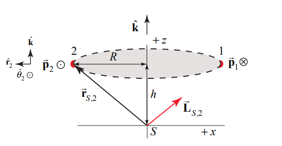
Para la partícula 1 (Figura 19.12), el momento angular alrededor del punto\(S\) es

\[\overrightarrow{\mathbf{L}}_{S, 1}=\overrightarrow{\mathbf{r}}_{S, 1} \times \overrightarrow{\mathbf{p}}_{1}=\left(R \hat{\mathbf{r}}_{1}+h \hat{\mathbf{k}}\right) \times m R \omega_{z} \hat{\mathbf{\theta}}_{1}=m R^{2} \omega_{z} \hat{\mathbf{k}}-h m R \omega_{z} \hat{\mathbf{r}}_{1} \nonumber \]

Para la partícula 2, (Figura 19.13), el momento angular alrededor del punto\(S\) es

\[\overrightarrow{\mathbf{L}}_{S, 2}=\overrightarrow{\mathbf{r}}_{S, 2} \times \overrightarrow{\mathbf{p}}_{2}=\left(R \hat{\mathbf{r}}_{2}+h \hat{\mathbf{k}}\right) \times m R \omega_{z} \hat{\mathbf{\theta}}_{2}=m R^{2} \omega_{z} \hat{\mathbf{k}}-h m R \omega_{z} \hat{\mathbf{r}}_{2} \nonumber \]

Debido a que las partículas se encuentran en lados opuestos del círculo,\(\hat{\mathbf{r}}_{1}=-\hat{\mathbf{r}}_{2}\). La suma vectorial solo apunta a lo largo del eje z y es igual a

\[\overrightarrow{\mathbf{L}}_{s}=\overrightarrow{\mathbf{L}}_{S, 1}+\overrightarrow{\mathbf{L}}_{S, 2}=2 m R^{2} \omega_{z} \hat{\mathbf{k}} \nonumber \]

Los dos vectores de momento angular se muestran en la Figura 19.14.

Figura 19.14 Momento angular sobre el punto\(S\) de ambas partículas y su suma

El momento de inercia de las dos partículas alrededor del eje z viene dado por\(I_{S}=2 m R^{2}\). Por lo tanto\(\overrightarrow{\mathbf{L}}_{S}=I_{S} \vec{\omega}\). El punto importante de este ejemplo es que los dos objetos están distribuidos simétricamente con respecto al eje z (lados opuestos de la órbita circular). Por lo tanto, el momento angular alrededor de cualquier punto\(S\) a lo largo del eje z tiene el mismo valor\(\overrightarrow{\mathbf{L}}_{s}=2 m r^{2} \omega \hat{\mathbf{k}}\) que es constante en magnitud y apunta en la dirección + z. Este resultado se generaliza a cualquier cuerpo rígido en el que la masa se distribuye simétricamente alrededor del eje de rotación.

Ejemplo\(\PageIndex{2}\): Angular Momentum of a System of Particles about Different Points

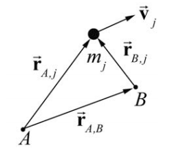
Considera un sistema de partículas de N, y dos puntos A y B (Figura 19.15). El momento angular de la\(j^{i h}\) partícula alrededor del punto A viene dado por

\[\overrightarrow{\mathbf{L}}_{A, j}=\overrightarrow{\mathbf{r}}_{A, j} \times m_{j} \overrightarrow{\mathbf{v}}_{j} \nonumber \]

Figura 19.15 Triángulo vectorial que relaciona la posición del objeto y los puntos A y B

El momento angular del sistema de partículas alrededor del punto A viene dado por la suma

\[\overrightarrow{\mathbf{L}}_{A}=\sum_{j=1}^{N} \overrightarrow{\mathbf{L}}_{A, j}=\sum_{j=1}^{N} \overrightarrow{\mathbf{r}}_{A, j} \times m_{j} \overrightarrow{\mathbf{v}}_{j} \nonumber \]

El momento angular alrededor del punto B se puede calcular de manera similar y viene dado por

\[\overrightarrow{\mathbf{L}}_{B}=\sum_{j=1}^{N} \overrightarrow{\mathbf{L}}_{B, j}=\sum_{j=1}^{N} \overrightarrow{\mathbf{r}}_{B, j} \times m_{j} \overrightarrow{\mathbf{v}}_{j} \nonumber \]

De la Figura 19.15, los vectores

\[\overrightarrow{\mathbf{r}}_{A, j}=\overrightarrow{\mathbf{r}}_{B, j}+\overrightarrow{\mathbf{r}}_{A, B} \nonumber \]

Podemos sustituir la Ecuación (19.5.14) por la Ecuación (19.5.12) rindiendo

\[\overrightarrow{\mathbf{L}}_{A}=\sum_{j=1}^{N}\left(\overrightarrow{\mathbf{r}}_{B, j}+\overrightarrow{\mathbf{r}}_{A, B}\right) \times m_{j} \overrightarrow{\mathbf{v}}_{j}=\sum_{j=1}^{N} \overrightarrow{\mathbf{r}}_{B, j} \times m_{j} \overrightarrow{\mathbf{v}}_{j}+\sum_{j=1}^{N} \overrightarrow{\mathbf{r}}_{A, B} \times m_{j} \overrightarrow{\mathbf{v}}_{j} \nonumber \]

El primer término en la Ecuación (19.5.15) es el momento angular alrededor del punto B. El vector\(\overrightarrow{\mathbf{r}}_{A, B}\) es una constante y así se puede sacar de la suma en el segundo término, y la Ecuación (19.5. 15) se convierte en

\[\overrightarrow{\mathbf{L}}_{A}=\overrightarrow{\mathbf{L}}_{B}+\overrightarrow{\mathbf{r}}_{A, B} \times \sum_{j=1}^{N} m_{j} \overrightarrow{\mathbf{v}}_{j} \nonumber \]

La suma en el segundo término es el impulso del sistema

\[\overrightarrow{\mathbf{p}}_{\mathrm{sys}}=\sum_{j=1}^{N} m_{j} \overrightarrow{\mathbf{v}}_{j} \nonumber \]

Por lo tanto, el momento angular alrededor de los puntos A y B están relacionados por

\[\overrightarrow{\mathbf{L}}_{A}=\overrightarrow{\mathbf{L}}_{B}+\overrightarrow{\mathbf{r}}_{A, B} \times \overrightarrow{\mathbf{p}}_{\mathrm{sys}} \nonumber \]

Por lo tanto, si el momento del sistema es cero, el momento angular es el mismo sobre cualquier punto.

\[\overrightarrow{\mathbf{L}}_{A}=\overrightarrow{\mathbf{L}}_{B}, \quad\left(\overrightarrow{\mathbf{p}}_{\mathrm{sys}}=\overrightarrow{\mathbf{0}}\right) \nonumber \]

En particular, el impulso de un sistema de partículas es cero por definición en el marco de referencia del centro de masa porque en ese marco de referencia\(\overrightarrow{\mathbf{p}}_{\mathrm{sys}}=\overrightarrow{\mathbf{0}}\). Por lo tanto, el momento angular es el mismo sobre cualquier punto en el marco de referencia del centro de masa.