9.5: Reflexiones múltiples (FABRY-PEROT)

Siempre que superpongamos dos ondas la distribución de intensidad tendrá la forma

$$I=I_{1}+I_{2}+2 \sqrt{I_{1} I_{2}} \cos \varphi \notag$$

Figura $\PageIndex{1}$: Inteferencias en una lámina delgada de índice $n$.

Figura $\PageIndex{2}$: Dispositivo real (izquierda) y dispositivo esquemático para el cálculo (derecha).

¿Y si superponemos una multitud de ondas en lugar de sólo dos?. No es difícil: podemos valernos de fenómenos de reflexión-refracción. Estamos haciendo una división de amplitud iterativa. Para obtener interferencia no hay más que reunir las ondas coherentes creadas. Si la fuente es puntual, basta utilizar una lente convergente para reunir las ondas en un punto del plano focal imagen. Si la fuente es extensa, las ondas planas interfieren automáticamente.

El vidrio no es una buena elección como material (el coeficiente de reflexión es muy pequeño, por lo que sólo la primera onda transmitida es suficientemente intensa, y la visibilidad es mala cuando se suman ondas de amplitudes muy dispares). Podemos o bien incidir de forma rasante, o bien introducir medios absorbentes, que es la idea que subyace al interferómetro de FABRY-PEROT.

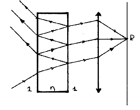
Disponemos dos espejos enfrentados entre sí, de material metálico y muy delgados para que haya suficiente transmisión. Habitualmente estas láminas van montadas sobre láminas de vidrio. Como las reflexiones en el vidrio son pequeñas, en lo que sigue sólo consideraremos las láminas metálicas, esquematizando el dispositivo como se ve en la figura 9.17. Si los coeficientes de reflexión son $r_{1}$ y $r_{2}$ y los de transmisión $t_{1}$ y $t_{2}$, la primera onda incidente sobre la pantalla es

$$t_{1} t_{2} A \notag$$

Figura $\PageIndex{3}$:Diagrama de los rayos


Figura 9.18: Diagrama de los rayos

la segunda onda es

$$t_{1} t_{2} r_{1} r_{2} A e^{i \phi} \notag$$

La diferencia de fase es

$$\phi=\frac{2 \pi}{\lambda}\left(2 n \Delta_{1}-n^{\prime} \Delta_{2}\right) \notag$$

$\left(2 n \Delta_{1}\right.$ es el camino óptico dentro del interferómetro). En términos de constantes del problema

$$\begin{aligned} \Delta_{1} &=\frac{d}{\cos \theta} \\ \Delta_{2} &=\Delta_{3} \sin \theta^{\prime} \\ \Delta_{3} &=2 \Delta_{1} \sin \theta \end{aligned}$$

$$\Delta_{2}=2 \frac{d}{\cos \theta} \sin \theta \sin \theta^{\prime} \notag$$

Como en cualquiera de las superficies paralelas a los espejos, dentro y fuera se deben verificar las condiciones de contorno (la proyección del vector de ondas se conserva)

$$\frac{\omega}{c} n \sin \theta=\ldots=\frac{\omega}{c} n^{\prime} \sin \theta^{\prime} \notag$$

es decir, la ley de SNELL: $n^{\prime} \sin \theta^{\prime}=n \sin \theta$. Finalmente

$$\Delta_{2}=2 \frac{d}{\cos \theta} \frac{n}{n^{\prime}} \sin ^{2} \theta \notag$$

y la diferencia de fase, al sustituir $\Delta_{1}$ y $\Delta_{2}$ vale

$$\phi=\ldots=\frac{2 \pi}{\lambda} 2 n d \cos \theta \notag$$

expresada en términos del índice de refracción del interferómetro, el ángulo de incidencia y la distancia entre los espejos. Obsérvese que es la misma expresión que la del interferómetro de MICHELSON.

Para las ondas sucesivas no hay más que aprovechar estos resultados. Por ejemplo, para la tercera,

$$t_{1} t_{2}\left(r_{1} r_{2}\right)^{2} A e^{i 2 \phi} \notag$$

De modo que la amplitud total debe ser una suma

$$\begin{aligned} A^{\prime} &=\sum_{m=0}^{\infty} t_{1} t_{2}\left(r_{1} r_{2}\right)^{m} e^{i m \phi} \\ &=\frac{t_{1} t_{2}}{1-r_{1} r_{2} e^{i \phi}} A \end{aligned}$$

(es una serie geométrica). Pero estamos interesados en la intensidad emergente $I^{\prime} \propto\left|A^{\prime}\right|^{2}$. Para hacerlo escribimos el número complejo

$$r_{1} r_{2}=\left|r_{1} r_{2}\right| e^{i 2 \delta} \notag$$

Como $I^{\prime}=\mathcal{T} I$

$$\mathcal{T}=\frac{\left|A^{\prime}\right|^{2}}{|A|^{2}}=\frac{I^{\prime}}{I}=\frac{\mathcal{T}_{\max }}{1+F \sin ^{2} \varphi} \notag$$

donde

$$\begin{aligned} \mathcal{T}_{\max } &=\frac{\left|t_{1} t_{2}\right|^{2}}{\left(1-\left|r_{1} r_{2}\right|\right)^{2}} \\ F &=\left(\frac{2 \sqrt{\left|r_{1} r_{2}\right|}}{1-\left|r_{1} r_{2}\right|}\right)^{2} \end{aligned}$$

son parámetros que sólo dependen del interferómetro, y

$$\begin{aligned} \varphi=& \frac{\phi}{2}+\delta=\\ \frac{2 \pi}{\lambda} n d \cos \theta+\delta \end{aligned}$$

es la fase. 9 Interferencia

Figura $\PageIndex{4}$: Función $\mathcal{T}(\varphi)$

• 9.5.1: Conclusiones

• 9.5.2: Tratamiento cuantitativo de la distribución de intensidad

• 9.5.3: Aplicaciones