
5.3: Ejercicios
- Page ID
- 87123

\( \newcommand{\vecs}[1]{\overset { \scriptstyle \rightharpoonup} {\mathbf{#1}} } \)
\( \newcommand{\vecd}[1]{\overset{-\!-\!\rightharpoonup}{\vphantom{a}\smash {#1}}} \)
\( \newcommand{\id}{\mathrm{id}}\) \( \newcommand{\Span}{\mathrm{span}}\)
( \newcommand{\kernel}{\mathrm{null}\,}\) \( \newcommand{\range}{\mathrm{range}\,}\)
\( \newcommand{\RealPart}{\mathrm{Re}}\) \( \newcommand{\ImaginaryPart}{\mathrm{Im}}\)
\( \newcommand{\Argument}{\mathrm{Arg}}\) \( \newcommand{\norm}[1]{\| #1 \|}\)
\( \newcommand{\inner}[2]{\langle #1, #2 \rangle}\)
\( \newcommand{\Span}{\mathrm{span}}\)
\( \newcommand{\id}{\mathrm{id}}\)
\( \newcommand{\Span}{\mathrm{span}}\)
\( \newcommand{\kernel}{\mathrm{null}\,}\)
\( \newcommand{\range}{\mathrm{range}\,}\)
\( \newcommand{\RealPart}{\mathrm{Re}}\)
\( \newcommand{\ImaginaryPart}{\mathrm{Im}}\)
\( \newcommand{\Argument}{\mathrm{Arg}}\)
\( \newcommand{\norm}[1]{\| #1 \|}\)
\( \newcommand{\inner}[2]{\langle #1, #2 \rangle}\)
\( \newcommand{\Span}{\mathrm{span}}\) \( \newcommand{\AA}{\unicode[.8,0]{x212B}}\)
\( \newcommand{\vectorA}[1]{\vec{#1}} % arrow\)
\( \newcommand{\vectorAt}[1]{\vec{\text{#1}}} % arrow\)
\( \newcommand{\vectorB}[1]{\overset { \scriptstyle \rightharpoonup} {\mathbf{#1}} } \)
\( \newcommand{\vectorC}[1]{\textbf{#1}} \)
\( \newcommand{\vectorD}[1]{\overrightarrow{#1}} \)
\( \newcommand{\vectorDt}[1]{\overrightarrow{\text{#1}}} \)
\( \newcommand{\vectE}[1]{\overset{-\!-\!\rightharpoonup}{\vphantom{a}\smash{\mathbf {#1}}}} \)
\( \newcommand{\vecs}[1]{\overset { \scriptstyle \rightharpoonup} {\mathbf{#1}} } \)
\( \newcommand{\vecd}[1]{\overset{-\!-\!\rightharpoonup}{\vphantom{a}\smash {#1}}} \)
Ejercicio\(\PageIndex{1}\) Pitot tube
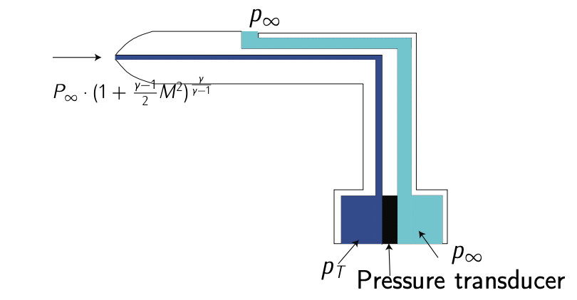
Figura Tubo Pitot de 5.19L.
Los aviones utilizan tubos pitot para medir la velocidad del aire. Consisten en un tubo que apunta directamente al flujo de fluido, de tal manera que el fluido en movimiento se pone en reposo (presión de estancamiento del aire,\(p_T\)). Típicamente, los tubos pitot incluyen también un puerto estático para medir la presión estática del aire (\(p_{\infty}\)). Ver Figura 5.19 como ilustración considerando el aire como un flujo compresible.
Considera las siguientes medidas a bordo de la aeronave:
- El tubo Pitot mide una presión de estancamiento\(p_T = 36975\ Pa\).
- La parte estática mide una presión estática de\(p_{\infty} = 22500\ Pa\).
Supongamos también que:
- el aire puede considerarse un gas ideal.
- el aire debe considerarse un fluido compresible. Para flujo compresible, uno tiene eso
\[P_T = P_{\infty} \cdot \left (1 + \dfrac{\gamma - 1}{2} M^2 \right )^{\tfrac{\gamma}{\gamma - 1}},\]
con\(\gamma = 1.4\) el coeficiente adiabático de aire, y\(M\) el número Mach:
\[M = \sqrt{V_{TAS}}{\sqrt{\gamma RT}}\]
Calcular la velocidad aerodinámica calibrada de la aeronave (CAS). 8
- Contestar
-
Observe que se puede aplicar la ecuación de Bernoulli a la línea de corriente del fluido dentro del tubo de Pitot. Suponiendo un flujo compresible, uno tiene:
\[P_T = P_{\infty} \cdot \left (1 + \dfrac{\gamma - 1}{2} M^2 \right )^{\tfrac{\gamma}{\gamma - 1}}.\]
Suponiendo que también el aire puede considerarse un gas ideal, se tiene:
\[P = \rho \cdot R \cdot T.\]
Además, se tiene la siguiente relación:
\[M = \dfrac{V_{TAS}}{\sqrt{\gamma RT}}.\]
Con todo, elaborando con estas tres ecuaciones, una tiene:
\[P_T = P_{\infty} \cdot \left (1 + \dfrac{\gamma - 1}{2} \dfrac{\rho_{\infty} \cdot V_{TAS}^2}{\gamma \cdot P_{\infty}} \right )^{\tfrac{\gamma}{\gamma - 1}}.\]
Considerar\(P_T - P_{\infty} = \Delta P\) y aislar\(V_{TAS}^2\):
\[V_{TAS}^2 = \dfrac{2\gamma}{\gamma - 1} \cdot \dfrac{P_{\infty}}{\rho_{\infty}} \left (\left (\dfrac{\Delta P}{P_{\infty}} + 1 \right )^{\tfrac{\gamma - 1}{\gamma}} - 1 \right ).\]
Sin embargo, se debe notar que solo con el tubo pitot y el puerto estático, no se pueden medir ni la temperatura ni la densidad. Así, no se\(V_{TAS}\) puede calcular directamente (necesitaríamos instrumentos/sensores adicionales). Esta es la razón detrás del concepto Calibrated Airspeed (CAS): la verdadera velocidad aérea que tendría una aeronave si volara con condiciones estándar del nivel medio del mar. Por lo tanto, CAS se define de la siguiente manera:
\[V_{CAS}^2 = \dfrac{2\gamma}{\gamma - 1} \cdot \dfrac{P_{MSL}}{\rho_{MSL}} \left (\left (\dfrac{\Delta P}{P_{MSL}} + 1 \right )^{\tfrac{\gamma - 1}{\gamma}} - 1 \right ).\label{eq5.3.8}\]
En efecto, la velocidad aerodinámica que se muestra en la cabina al piloto (denominada Velocidad Aérea Indicada) es la velocidad CAS corregida con errores del instrumento.
Ahora, entrando en la Eq. (\(\ref{eq5.3.8}\)) con los valores dados en el enunciado, se tiene la solución al problema:
\[V_{CAS} = 150\ m/s.\nonumber\]
8. supongamos que las condiciones medias del nivel del mar son las estándar según ISA,\(P_{MSL} = 101325\ Pa\) y\(\rho_{MSL} = 1.225\ kg/m^3\)