1.5: Raíces de números complejos

Recordemos que si\(z=x+iy\) es un número complejo distinto de cero, entonces se puede escribir en forma polar como

\(z=r(cosθ+isinθ)\)

donde\(r=\sqrt{x^{2}+y^{2}}\) y\(\theta \) es el ángulo, en radianes, desde el eje x positivo hasta el rayo que conecta el origen con el punto\(z\).

Ahora bien, la fórmula de de Moivre establece que si\(z=r(cosθ+isinθ)\) y\(n\) es un entero positivo, entonces

\(z^{n}=r^{n}(cosn\theta +isinn\theta )\)

Dejar\(w\) ser un número complejo. Usar la fórmula de Moivre nos ayudará a resolver la ecuación

\(z^{n}=w\)

para\(z\) cuando\(w\) se da.

Supongamos que\(w=r(cosθ+isinθ)\) y\(z=\rho(cos\psi +isin\psi )\) Entonces la fórmula de Moivre da

\(z^{n}=\rho ^{n}(cosn\psi +isinn\psi )\)

De ello se deduce que

\(\rho ^{n}=r=\left | w \right |\)

por la singularidad de la representación polar y

\(n\Psi =\theta +k(2\pi )\),

donde\(k\) es algún número entero. Así

\(z=\sqrt[n]{r}[cos(\frac{\theta }{n}+\frac{2k\pi }{n})+isin(\frac{\theta }{n}+\frac{2k\pi }{n})]\).

Cada valor de\(k=0,1,2,…,n−1\) da un valor diferente de\(z\). Cualquier otro valor de\(k\) simplemente repite uno de los valores de\(z\) correspondiente a\(k=0,1,2,…,n−1\). Por lo tanto, hay\(n\) exactamente las raíces de un número complejo distinto de cero.

Usando la fórmula de Euler:

\(e^{i\theta }=cos\theta +isin\theta \),

el número complejo también se\(z=r(cos\theta +isin\theta) \\) puede escribir en forma exponencial como

\(z=re^{i\theta }\)

Por lo tanto, las raíces\(n\) th de un número complejo distinto de cero también se\(z≠0\) pueden expresar como

\ (\ begin {eqnarray}\ label {expform}
z=\ sqrt [n] {r}\;\ mbox {exp}\ izquierda [i\ left (\ frac {\ theta} {n} +\ frac {2k\ pi} {n}\ derecha)\ derecha]
\ end {eqnarray}\)

donde\(k=0,1,2,...,n-1\).

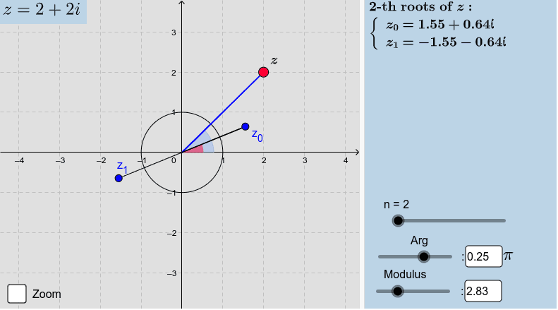
El applet a continuación muestra una representación geométrica de las raíces\(n\) th de un número complejo, hasta\(n=10\). Arrastre el punto rojo alrededor para cambiar el valor de\(z\) o arrastre los controles deslizantes.

Código

Ingresa el siguiente script en GeoGebra para explorarlo tú mismo y hacer tu propia versión. El símbolo # indica comentarios.

#Complex number
    
Z = 1 + ί

#Modulus of Z

r = abs(Z)

#Angle of Z

theta = atan2(y(Z), x(Z))

#Number of roots

n = Slider(2, 10, 1, 1, 150, false, true, false, false)

#Plot n-roots

nRoots = Sequence(r^(1 / n) * exp(  ί * ( theta / n + 2 * pi * k / n ) ), k, 0, n-1)

---

Ejercicio\(\PageIndex{1}\)

A partir de la forma exponencial (1) de las raíces, muestran que todas las raíces\(n\) th se encuentran en el círculo\(\left | z \right |=\sqrt[n]{r}\) alrededor del origen y están igualmente espaciadas cada\(\frac{2\pi }{n}\) radianes, comenzando por el argumento\(\frac{\theta }{n}\).