4.2: Integración compleja

La magia y el poder del cálculo se basa en última instancia en el asombroso hecho de que la diferenciación y la integración son operaciones mutuamente inversas. Y, así como las funciones complejas disfrutan de notables propiedades de diferenciabilidad no compartidas por sus contrapartes reales, así la belleza sublime de la integración compleja va mucho más allá de su progenitor real.

Peter Oliver

Contorno integral

Considera un contorno\(C\) parametrizado por\(z(t)=x(t)+iy(t)\) for\(a≤t≤b\). Definimos la integral de la función compleja\(C\) a lo largo de ser el número complejo

\(\int_{C}f(z)dz=\int_{a}^{b}f\left ( z\left ( t \right ) \right ){z}'\left ( t \right )dt\). (1)

Aquí asumimos que\(f(z(t))\) es continuo por tramos en el intervalo\(\) a≤t≤b y nos referimos a la función\(\) f (z) como continua por tramos en\(C\). Dado que\(C\) es un contorno, también\(z′(t)\) es continuo por partes\(a≤t≤b\); y así se asegura la existencia de integral (1).

El lado derecho de (1) es una integral real ordinaria de una función de valor complejo; es decir, si\(w(t)=u(t)+iv(t)\), entonces

\(\int_{a}^{b}w\left ( t \right )dt=\int_{a}^{b}u\left ( t \right )dt+i\int_{a}^{b}v\left ( t \right )dt\)(2)

Ahora escribamos el integrand

\(f(z)=u(x,y)+iv(x,y)\)

en términos de sus partes reales e imaginarias, así como el diferencial

\(dz=\frac{dz}{dt}dt=\left ( \frac{dx}{dt} +i\frac{dy}{dt}\right )dt=dx+idy\)

Luego, la integral compleja (1) se divide en un par de integrales de línea reales:

\(\int_{C}f\left ( z \right )dz=\int_{C}\left ( u+iv \right )\left ( dx+idy \right )=\int_{C}\left ( udx-vdy \right )+i\int_{C}\left ( vdx+udy \right )\). (3)

Ejemplo\(\PageIndex{1}\)

Vamos a evaluar\(\int_{C}f\left ( \bar{z} \right )dz\), donde\(C\) se da por\(x=3t\),\(y=t^{2}\),\(y=t^{2}\), con\(−1≤t≤4\).

Figura 1:\(\), con\(−1≤t≤4\).

Aquí tenemos que\(C\) es\(z\left ( t \right )=3t+it^{2}\). Por lo tanto, con la identificación\(f\left ( z \right )=\bar{z}\) que tenemos

\(f\left ( z\left ( t \right ) \right )=\overline{3t+it^{2}}=3t-it^{2}\).

También,\(z′(t)=3+2it\), y así la integral es

\(\int_{C}\bar{z}dz=\int_{-1}^{4}\left ( 3t-it^{2} \right )\left ( 3+2it \right )dt\\=\int_{-1}^{4}\left ( 2t^{3}+9t+3t^{2}i \right )dt\\=\int_{-1}^{4}\left ( 2t^{3}+9t \right )dt+i\int_{-1}^{4}3t^{2}dt\\=\left.\left ( \frac{1}{2} t^{4}+\frac{9}{2}t^{2}\right )\right|_{-1}^{4}+\left.it^{3} \right |_{-1}^{4}\\=195+65i\).

Ejemplo\(\PageIndex{2}\)

Ahora vamos a evaluar\(\int_{C}^{}\frac{1}{z}dz\), dónde\(C\) está el círculo\(x=cos\,t\),\(y=sin\,t\), con\(0\leq t\leq 2\pi \).

Figura 2:\(C:z\left ( t \right )=cos\,t+i\,sin\,t=e^{it}\), con\(0\leq t\leq 2\pi\).

En este caso\(C\) es\(z\left ( t \right )=cos\,t+i\,sin\,t=e^{it}\),

\(f\left ( z\left ( t \right ) \right )=\frac{1}{e^{it}}\)

y,\({z}'\left ( t \right )=ie^{it}\). Así

\(\int_{C}^{}\frac{1}{z}dz=\int_{0}^{2\pi }\left ( e^{-it} \right )ie^{it}dt=i\int_{0}^{2\pi }dt=2\pi i\).

---

Evaluación numérica de integrales complejas

Exploración 1

Utilice el siguiente applet para explorar numéricamente la integral

\(\int_{C}\bar{z}dz\)

con diferentes contornos\(C\):

• Segmentos de línea.
• Semicírculos.
• Círculos, orientados positiva y negativamente.

También puede cambiar la opción de trazado del color del dominio. Arrastre los puntos alrededor y observe cuidadosamente lo que sucede. Entonces resuelve el Ejercicio 1 a continuación.

GRAFO INTERACTIVO

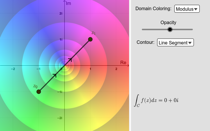
Las flechas en los contornos indican la dirección.

Ejercicio\(\PageIndex{1}\)

Ejercicio 1: Utilice la definición (1) para evaluar\(\int_{C}\bar{z}dz\), para los siguientes contornos\(C\) de\(z_{0}=-2i\) a\(z_{1}=2i\):

1. Segmento de línea. Es decir,\(z\left ( t \right )=-2i\left ( 1-t \right )+2it\), con\(0≤t≤1\).
2. Semicírculo derecho. Es decir,\(z\left ( \theta  \right )=2e^{i\theta }\) con\(-\frac{\pi }{2}\leq \theta \leq \frac{\pi }{2}\).
3. Semicírculo izquierdo. Es decir,\(z\left ( \theta  \right )=-2e^{-i\theta }\) con\(0\leq \theta \leq \pi \).

Usa el applet para confirmar tus resultados.

¿Qué conclusiones (si las hay) puedes sacar sobre la función\(\bar{z}\) a partir de esto?

Exploración 2

Ahora usa el applet a continuación para explorar numéricamente las integrales

\(\int_{C}^{}\left ( z^{2}+z \right )dz\);\(\int_{C}^{}\frac{1}{z^{2}}dz\)

con diferentes contornos\(C\) (segmentos de línea, semicírculos y círculos). Arrastre los puntos alrededor y observe cuidadosamente lo que sucede. Puede seleccionar las funciones z^2+z o 1/z^2 de la lista en la esquina superior izquierda. Después resuelve los Ejercicios 2 y 3.

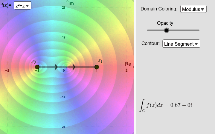
Ejercicio\(\PageIndex{2}\)

Ejercicio 2: Considerar la integral

\(I_{1}=\int_{C}^{}\left ( z^{2} +z\right )dz\).

Utilice el applet para analizar el valor de\(I_{1}\) en los siguientes casos:

1. \(C\)es cualquier contorno de\(z_{0}=-1-i\) a\(z_{1}=1+i\).
2. \(C\)es el círculo con centro\(z_{0}\) y radio\(r>0\),\(\left | z-z_{0} \right |=r\); orientado positiva o negativamente. En estos casos, seleccione Circulo o Circulo de la barra de

¿Qué conclusiones (si las hay) puedes sacar sobre el valor\(I_{1}\) y la función\(z^{2}+z\) de esto?

Ejercicio\(\PageIndex{3}\)

Ejercicio 3: Ahora considerando integral

\(I_{2}=\int_{C}^{}\frac{1}{z^{2}}dz\).

Primero, en el applet selecciona la función f (z) =1/z^2. Luego analice los valores de\(I_{2}\) en los siguientes casos:

1. \(C\)es cualquier contorno de\(z_{0}=-i\) a\(z_{1}=i\). ¿Qué sucede cuando selecciona Segmento de línea en el applet? ¿Qué sucede cuando seleccionas Semicírculos?
2. \(C\)es el círculo con centro\(z_{0}\) y radio\(r>0\),\(\left | z-z_{0} \right |=r\); orientado positiva o negativamente. En este caso, seleccione Círculo o Círculo: ¿Qué pasa si\(z=0\) está dentro o fuera del círculo? ¿Qué pasa si\(z=0\) se encuentra en el contorno, por ejemplo cuando\(\(z_{0}=1\)\) y\(r=1\)?

¿Qué conclusiones (si las hay) puedes sacar sobre el valor\(I_{2}\) y la función\(\frac{1}{z^{2}}\) de esto?

---

Antiderivados

Si bien el valor de una integral de contorno de una función\(f(z)\) desde un punto fijo\(z_{0}\) a un punto fijo\(z_{1}\) depende, en general, de la ruta que se tome, existen ciertas funciones cuyas integrales desde\(z_{0}\) para\(z_{1}\) tener valores que son independientes de path, como has visto en Ejercicios 2 y 3. Estos ejemplos también ilustran el hecho de que los valores de integrales alrededor de caminos cerrados son a veces, pero no siempre, cero. El siguiente teorema es útil para determinar cuándo la integración es independiente de path y, además, cuando una integral alrededor de una trayectoria cerrada tiene valor cero. Esto se conoce como la versión compleja del Teorema Fundamental del Cálculo.

Teorema\(\PageIndex{1}\)

Dejar\(f(z)=F′(z)\) ser la derivada de una función compleja de valor único\(F(z)\) definida en un dominio\(\Omega \subset \mathbb{C}\). \(C\)Sea cualquier conteo que se encuentre completamente adentro\(\Omega\) con punto inicial\(z_{0}\) y punto final\(z_{1}\). Entonces

\(\int_{C}^{}f\left ( z \right )dz=\left.F\left ( z \right )  \right |_{z_{0}}^{z_{1}}=F\left ( z_{1} \right )-F\left ( z_{0} \right )\).

Prueba: Esto se desprende de la definición (1) y de la regla de la cadena. Eso es

\(\int_{C}^{}f\left ( z \right )dz=\int_{C}{F}'\left ( z\left ( t \right ) \right )\frac{dz}{dt}dt\\=\int_{a}^{b}\frac{d}{dt}F\left ( z\left ( t \right ) \right )dt\\=F\left ( z\left ( b \right ) \right )-F\left ( z\left ( a \right ) \right )\\=F\left ( z_{1} \right )-F\left ( z_{0} \right )\)

donde\(z_{0}=z_{a}\) y\(z_{1}=z_{b}\) son los puntos finales del contorno\(C\). ■