
5.1: Los fundamentos de la teoría gráfica
- Page ID
- 117101

Consulte la Sección 4.5 para revisar alguna terminología básica sobre las gráficas.
Una gráfica\(G\) consiste en un par\((V,E)\), donde\(V\) está el conjunto de vértices y\(E\) el conjunto de aristas. Escribimos\(V(G)\) para los vértices de\(G\) y\(E(G)\) para los bordes de\(G\) cuando sea necesario para evitar ambigüedades, como cuando hay más de una gráfica en discusión.
Si no hay dos bordes que tengan los mismos extremos decimos que no hay múltiples aristas, y si ningún borde tiene un solo vértice como ambos extremos decimos que no hay bucles. Una gráfica sin bucles y sin múltiples aristas es una gráfica simple. Una gráfica sin bucles, pero posiblemente con múltiples aristas es un multígrafo. La condensación de un multígrafo es la gráfica simple que se forma al eliminar múltiples aristas, es decir, eliminar todos menos uno de los bordes con los mismos extremos. Para formar la condensación de una gráfica, también se eliminan todos los bucles. A veces nos referimos a una gráfica como una gráfica general para enfatizar que la gráfica puede tener bucles o múltiples aristas.
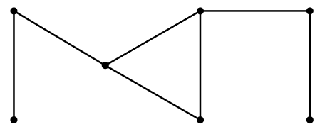
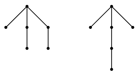
Los bordes de una gráfica simple se pueden representar como un conjunto de dos conjuntos de elementos; por ejemplo,\[(\{v_1,\ldots,v_7\},\{\{v_1,v_2\},\{v_2,v_3\},\{v_3,v_4\},\{v_3,v_5\}, \{v_4,v_5\},\{v_5,v_6\},\{v_6,v_7\}\})\nonumber \] es una gráfica que se puede representar como en la Figura\(\PageIndex{1}\). Esta gráfica también es una gráfica conectada: cada par de vértices\(v\),\(w\) está conectado por una secuencia de vértices y aristas,\(v=v_1,e_1,v_2,e_2,\ldots,v_k=w\), donde\(v_i\) y\(v_{i+1}\) son los puntos finales de borde\(e_{i}\). Las gráficas mostradas en la Figura 4.5.2 están conectadas, pero la figura podría interpretarse como una sola gráfica que no está conectada.
Un gráfico\(G=(V,E)\) que no es simple se puede representar mediante el uso de multiconjuntos: un bucle es un multiconjunto\(\{v,v\}=\{2\cdot v\}\) y múltiples bordes se representan haciendo\(E\) un multiconjunto. La condensación de un multígrafo se puede formar interpretando el multiconjunto\(E\) como un conjunto.
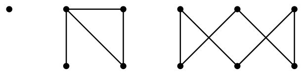
A general graph that is not connected, has loops, and has multiple edges is shown in Figure \(\PageIndex{2}\). The condensation of this graph is shown in Figure \(\PageIndex{3}\).
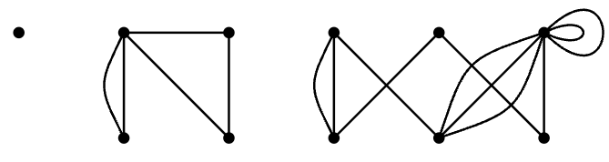
The degree of a a vertex \(v\), \(d(v)\), is the number of times it appears as an endpoint of an edge. If there are no loops, this is the same as the number of edges incident with \(v\), but if \(v\) is both endpoints of an edge, namely, of a loop, then this contributes 2 to the degree of \(v\). The degree sequence of a graph is a list of its degrees; the order does not matter, but usually we list the degrees in increasing or decreasing order. The degree sequence of the graph in Figure \(\PageIndex{2}\), listed clockwise starting at the upper left, is \(0,4,2,3,2,8,2,4,3,2,2\). We typically denote the degrees of the vertices of a graph by \(d_i\), \(i=1,2,\ldots,n\), where \(n\) is the number of vertices. Depending on context, the subscript \(i\) may match the subscript on a vertex, so that \(d_i\) is the degree of \(v_i\), or the subscript may indicate the position of \(d_i\) in an increasing or decreasing list of the degrees; for example, we may state that the degree sequence is \(d_1\le d_2\le \cdots\le d_n\).
Our first result, simple but useful, concerns the degree sequence.
In any graph, the sum of the degree sequence is equal to twice the number of edges, that is, \[\sum_{i=1}^n d_i = 2|E|.\nonumber \]
- Proof
-
Let \(d_i\) be the degree of \(v_i\). The degree \(d_i\) counts the number of times \(v_i\) appears as an endpoint of an edge. Since each edge has two endpoints, the sum \(\sum_{i=1}^n d_i\) counts each edge twice.
An easy consequence of this theorem:
An interesting question immediately arises: given a finite sequence of integers, is it the degree sequence of a graph? Clearly, if the sum of the sequence is odd, the answer is no. If the sum is even, it is not too hard to see that the answer is yes, provided we allow loops and multiple edges. The sequence need not be the degree sequence of a simple graph; for example, it is not hard to see that no simple graph has degree sequence \(0,1,2,3,4\). A sequence that is the degree sequence of a simple graph is said to be graphical. Graphical sequences have be characterized; the most well known characterization is given by this result:
A sequence \(d_1\ge d_2\ge \ldots\ge d_n\) is graphical if and only if \(\sum_{i=1}^n d_i\) is even and for all \(k\in \{1,2,\ldots,n\}\), \[\sum_{i=1}^k d_i\le k(k-1)+\sum_{i=k+1}^n \min(d_i,k).\nonumber \]
It is not hard to see that if a sequence is graphical it has the property in the theorem; it is rather more difficult to see that any sequence with the property is graphical.
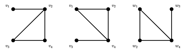
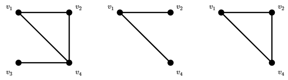
What does it mean for two graphs to be the same? Consider these three graphs: \[\eqalign{ G_1&=(\{v_1,v_2,v_3,v_4\},\{\{v_1,v_2\},\{v_2,v_3\},\{v_3,v_4\},\{v_2,v_4\}\})\cr G_2&=(\{v_1,v_2,v_3,v_4\},\{\{v_1,v_2\},\{v_1,v_4\},\{v_3,v_4\},\{v_2,v_4\}\})\cr G_3&=(\{w_1,w_2,w_3,w_4\},\{\{w_1,w_2\},\{w_1,w_4\},\{w_3,w_4\},\{w_2,w_4\}\})\cr }\nonumber \] These are pictured in Figure \(\PageIndex{4}\). Simply looking at the lists of vertices and edges, they don't appear to be the same. Looking more closely, \(G_2\) and \(G_3\) are the same except for the names used for the vertices: \(v_i\) in one case, \(w_i\) in the other. Looking at the pictures, there is an obvious sense in which all three are the same: each is a triangle with an edge (and vertex) dangling from one of the three vertices. Although \(G_1\) and \(G_2\) use the same names for the vertices, they apply to different vertices in the graph: in \(G_1\) the "dangling'' vertex (officially called a pendant vertex) is called \(v_1\), while in \(G_2\) it is called \(v_3\). Finally, note that in the figure, \(G_2\) and \(G_3\) look different, even though they are clearly the same based on the vertex and edge lists.
So how should we define "sameness'' for graphs? We use a familiar term and definition: isomorphism.
Definition \(\PageIndex{1}\): Isomorphic & Isomorphism
Suppose \(G_1=(V,E)\) and \(G_2=(W,F)\). \(G_1\) and \(G_2\) are isomorphic if there is a bijection \(f\colon V\to W\) such that \(\{v_1,v_2\}\in E\) if and only if \(\{f(v_1),f(v_2)\}\in F\). In addition, the repetition numbers of \(\{v_1,v_2\}\) and \(\{f(v_1),f(v_2)\}\) are the same if multiple edges or loops are allowed. This bijection \(f\) is called an isomorphism. When \(G_1\) and \(G_2\) are isomorphic, we write \(G_1\cong G_2\).
Each pair of graphs in Figure \(\PageIndex{4}\) are isomorphic. For example, to show explicitly that \(G_1\cong G_3\), an isomorphism is \[\eqalign{ f(v_1)&=w_3\cr f(v_2)&=w_4\cr f(v_3)&=w_2\cr f(v_4)&=w_1.\cr }\nonumber \]
Clearly, if two graphs are isomorphic, their degree sequences are the same. The converse is not true; the graphs in Figure \(\PageIndex{5}\) both have degree sequence \(1,1,1,2,2,3\), but in one the degree-2 vertices are adjacent to each other, while in the other they are not. In general, if two graphs are isomorphic, they share all "graph theoretic'' properties, that is, properties that depend only on the graph. As an example of a non-graph theoretic property, consider "the number of times edges cross when the graph is drawn in the plane.''
In a more or less obvious way, some graphs are contained in others.
Definition \(\PageIndex{2}\): Subgraph & Induced Subgraph
Graph \(H=(W,F)\) is a subgraph of graph \(G=(V,E)\) if \(W\subseteq V\) and \(F\subseteq E\). (Since \(H\) is a graph, the edges in \(F\) have their endpoints in \(W\).) \(H\) is an induced subgraph if \(F\) consists of all edges in \(E\) with endpoints in \(W\). See Figure \(\PageIndex{6}\). Whenever \(U\subseteq V\) we denote the induced subgraph of \(G\) on vertices \(U\) as \(G[U]\).
A path in a graph is a subgraph that is a path; if the endpoints of the path are \(v\) and \(w\) we say it is a path from \(v\) to \(w\). A cycle in a graph is a subgraph that is a cycle. A clique in a graph is a subgraph that is a complete graph.
If a graph \(G\) is not connected, define \(v\sim w\) if and only if there is a path connecting \(v\) and \(w\). It is not hard to see that this is an equivalence relation. Each equivalence class corresponds to an induced subgraph \(G\); these subgraphs are called the connected components of the graph.