5.8: Colorear Gráfica

Como discutimos brevemente en la Sección 1.2, el problema de coloración gráfica más famoso es sin duda el problema de coloración del mapa, propuesto en el siglo XIX y finalmente resuelto en 1976.

Definición\(\PageIndex{1}\): A Proper Coloring

Una coloración adecuada de una gráfica es una asignación de colores a los vértices de la gráfica para que no haya dos vértices adyacentes del mismo color.

Por lo general, dejamos caer la palabra “apropiado” a menos que otros tipos de coloración también estén bajo discusión. Por supuesto, los “colores” no tienen que ser colores reales; pueden ser cualquier etiqueta distinta—enteros, por ejemplo. Si una gráfica no está conectada, cada componente conectado se puede colorear de forma independiente; salvo que se indique lo contrario, suponemos que las gráficas están conectadas. También asumimos que las gráficas son simples en esta sección.

La coloración gráfica tiene muchas aplicaciones además de su interés intrínseco.

Ejemplo\(\PageIndex{1}\)

Si los vértices de una gráfica representan clases académicas, y dos vértices son adyacentes si las clases correspondientes tienen personas en común, entonces se puede usar una coloración de los vértices para programar reuniones de clase. Aquí los colores serían horarios de horario, como 8MWF, 9MWF, 11Tth, etc.

Ejemplo\(\PageIndex{2}\)

Si los vértices de una gráfica representan estaciones de radio, y dos vértices son adyacentes si las estaciones están lo suficientemente cerca como para interferir entre sí, se puede usar una coloración para asignar frecuencias no interferentes a las estaciones.

Ejemplo\(\PageIndex{3}\)

Si los vértices de una gráfica representan señales de tráfico en una intersección, y dos vértices son adyacentes si las señales correspondientes no pueden ser verdes al mismo tiempo, se puede usar una coloración para designar conjuntos de señales que pueden ser verdes al mismo tiempo.

La coloración gráfica está estrechamente relacionada con el concepto de un conjunto independiente.

Definición\(\PageIndex{2}\): Independent

Un conjunto\(S\) de vértices en una gráfica es independiente si no hay dos vértices de\(S\) adyacentes.

Si una gráfica está coloreada correctamente, los vértices a los que se les asigna un color particular forman un conjunto independiente. Dada una gráfica\(G\) es fácil encontrar una coloración adecuada: darle a cada vértice un color diferente. Claramente la cantidad interesante es el número mínimo de colores requeridos para una coloración. También es fácil encontrar conjuntos independientes: simplemente elija vértices que no sean mutuamente adyacentes. Un solo conjunto de vértices, por ejemplo, es independiente, y por lo general es fácil encontrar conjuntos independientes más grandes. La cantidad interesante es el tamaño máximo de un conjunto independiente.

Definición\(\PageIndex{3}\): Chromatic Number

El número cromático de una gráfica\(G\) es el número mínimo de colores requeridos en una coloración adecuada; se denota\(\chi(G)\). El número de independencia de\(G\) es el tamaño máximo de un conjunto independiente; se denota\(\alpha(G)\).

La primera pregunta natural sobre estos parámetros gráficos es: qué tan pequeños o grandes pueden ser en una gráfica\(G\) con\(n\) vértices. Es fácil ver que

\[\eqalign{ 1&\le \chi(G)\le n\cr 1&\le \alpha(G)\le n\cr }\nonumber \]

y que todos los límites son alcanzables: Una gráfica sin aristas tiene número cromático 1 y número de independencia\(n\), mientras que una gráfica completa tiene número cromático\(n\) y número de independencia 1. Estas desigualdades, pues, no son muy interesantes. Veremos algunos que son más interesantes.

Otra pregunta natural: ¿Cuál es la relación entre el número cromático de una gráfica\(G\) y el número cromático de una subgrafía de\(G\)? Esto también es simple, pero bastante útil a veces.

Teorema \(\PageIndex{1}\)

Si\(H\) es un subgrafo de\(G\),\(\chi(H)\le \chi(G)\).

Prueba

Cualquier coloración de\(G\) proporciona una coloración adecuada de\(H\), simplemente asignando los mismos colores a vértices de los\(H\) que tienen en\(G\). Esto significa que se\(H\) puede colorear con\(\chi(G)\) colores, quizás incluso menos, que es exactamente lo que queremos.

A menudo este hecho es interesante “a la inversa”. Por ejemplo, si\(G\) tiene una subgrafía\(H\) que es una gráfica completa\(K_m\), entonces\(\chi(H)=m\) y así\(\chi(G)\ge m\). Un subgrafo de\(G\) eso es una gráfica completa se llama camarilla, y hay un parámetro gráfico asociado.

Definición\(\PageIndex{4}\): Clique Number

El número de camarilla de una gráfica\(G\) es el más grande\(m\) tal que\(K_m\) es un subgrafo de\(G\).

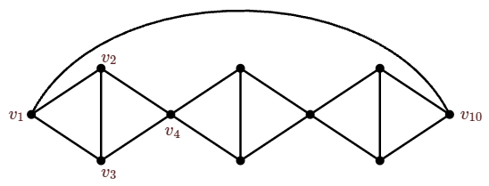
Es tentador especular que la única forma en que una gráfica\(G\) podría requerir\(m\) colores es teniendo tal subgrafía. Esto es falso; las gráficas pueden tener un número cromático alto mientras que tienen un número bajo de camarilla; ver Figura\(\PageIndex{1}\). Es fácil ver que esta gráfica tiene\(\chi\ge 3\), porque hay muchas 3 camarillas en la gráfica. En general puede ser difícil mostrar que una gráfica no se puede colorear con un número dado de colores, pero en este caso es fácil ver que la gráfica de hecho no se puede colorear con tres colores, porque tanto es “forzado”. Supongamos que la gráfica puede ser coloreada con 3 colores. Comenzando por la izquierda si el vértice\(v_1\) obtiene el color 1, entonces\(v_2\) y\(v_3\) debe ser coloreado 2 y 3, y el vértice\(v_4\) debe ser el color 1. Continuando,\(v_{10}\) debe ser el color 1, pero esto no está permitido, entonces\(\chi>3\). Por otro lado, ya que se\(v_{10}\) puede colorear 4, vemos\(\chi=4\).

Paul Erdős demostró en 1959 que hay gráficas con número cromático arbitrariamente grande y contorno arbitrariamente grande (la cincha es el tamaño del ciclo más pequeño en una gráfica). Esto es mucho más fuerte que la existencia de gráficas con alto número cromático y bajo número de camarilla.

Figura\(\PageIndex{1}\): Gráfica con camarilla número 3 y número cromático 4.

Las gráficas bipartitas con al menos un borde tienen el número cromático 2, ya que las dos partes son cada una conjuntos independientes y se pueden colorear con un solo color. Por el contrario, si una gráfica puede ser de 2 colores, es bipartita, ya que todos los bordes conectan vértices de diferentes colores. Esto significa que es fácil identificar gráficas bipartitas: Colorea cualquier vértice con el color 1; colorear a sus vecinos color 2; continuar de esta manera coloreará o no con éxito la gráfica completa con 2 colores. Si falla, la gráfica no puede ser de 2 colores, ya que todas las opciones para los colores de vértice son forzadas.

If a graph is properly colored, then each color class (a color class is the set of all vertices of a single color) is an independent set.

Theorem \(\PageIndex{2}\)

In any graph \(G\) on \(n\) vertices, \( {n\over \alpha}\le\chi\).

Proof

Suppose \(G\) is colored with \(\chi\) colors. Since each color class is independent, the size of any color class is at most \(\alpha\). Let the color classes be \(V_1,V_2,\ldots,V_\chi\). Then \[ n=\sum_{i=1}^\chi |V_i| \le \chi\alpha, \nonumber\] as desired.

We can improve the upper bound on \(\chi(G)\) as well. In any graph \(G\), \(\Delta(G)\) is the maximum degree of any vertex.

Theorem \(\PageIndex{3}\)

In any graph \(G\), \( \chi\le\Delta+1\).

Proof

We show that we can always color \(G\) with \(\Delta+1\) colors by a simple greedy algorithm: Pick a vertex \(v_n\), and list the vertices of \(G\) as \(v_1,v_2,\ldots,v_n\) so that if \(i< j\), \(\text{d}(v_i,v_n) \ge\text{d}(v_j,v_n)\), that is, we list the vertices farthest from \(v_n\) first. We use integers \(1,2,\ldots, \Delta+1\) as colors. Color \(v_1\) with 1. Then for each \(v_i\) in order, color \(v_i\) with the smallest integer that does not violate the proper coloring requirement, that is, which is different than the colors already assigned to the neighbors of \(v_i\). For \(i< n\), we claim that \(v_i\) is colored with one of \(1,2,\ldots,\Delta\).

This is certainly true for \(v_1\). For \(1< i< n\), \(v_i\) has at least one neighbor that is not yet colored, namely, a vertex closer to \(v_n\) on a shortest path from \(v_n\) to \(v_i\). Thus, the neighbors of \(v_i\) use at most \(\Delta-1\) colors from the colors \(1,2,\ldots,\Delta\), leaving at least one color from this list available for \(v_i\).

Once \(v_1,\ldots,v_{n-1}\) have been colored, all neighbors of \(v_n\) have been colored using the colors \(1,2,\ldots,\Delta\), so color \(\Delta+1\) may be used to color \(v_n\).

Note that if \(\text{d}(v_n)< \Delta\), even \(v_n\) may be colored with one of the colors \(1,2,\ldots,\Delta\). Since the choice of \(v_n\) was arbitrary, we may choose \(v_n\) so that \(\text{d}(v_n)< \Delta\), unless all vertices have degree \(\Delta\), that is, if \(G\) is regular. Thus, we have proved somewhat more than stated, namely, that any graph \(G\) that is not regular has \(\chi\le\Delta\). (If instead of choosing the particular order of \(v_1,\ldots,v_n\) that we used we were to list them in arbitrary order, even vertices other than \(v_n\) might require use of color \(\Delta+1\). This gives a slightly simpler proof of the stated theorem.) We state this as a corollary.

Corollary \(\PageIndex{1}\)

If \(G\) is not regular, \(\chi\le\Delta\).

There are graphs for which \(\chi=\Delta+1\): any cycle of odd length has \(\Delta=2\) and \(\chi=3\), and \(K_n\) has \(\Delta=n-1\) and \(\chi=n\). Of course, these are regular graphs. It turns out that these are the only examples, that is, if \(G\) is not an odd cycle or a complete graph, then \(\chi(G)\le\Delta(G)\).

Theorem \(\PageIndex{4}\): Brook's Theorem

If \(G\) is a graph other than \(K_n\) or \(C_{2n+1}\), \(\chi\le \Delta\).

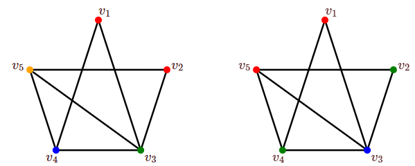
The greedy algorithm will not always color a graph with the smallest possible number of colors. Figure \(\PageIndex{2}\) shows a graph with chromatic number 3, but the greedy algorithm uses 4 colors if the vertices are ordered as shown.

Figure \(\PageIndex{2}\): A greedy coloring on the left and best coloring on the right.

In general, it is difficult to compute \(\chi(G)\), that is, it takes a large amount of computation, but there is a simple algorithm for graph coloring that is not fast. Suppose that \(v\) and \(w\) are non-adjacent vertices in \(G\). Denote by \(G+\{v,w\}=G+e\) the graph formed by adding edge \(e=\{v,w\}\) to \(G\). Denote by \(G/e\) the graph in which \(v\) and \(w\) are "identified'', that is, \(v\) and \(w\) are replaced by a single vertex \(x\) adjacent to all neighbors of \(v\) and \(w\). (But note that we do not introduce multiple edges: if \(u\) is adjacent to both \(v\) and \(w\) in \(G\), there will be a single edge from \(x\) to \(u\) in \(G/e\).)

Consider a proper coloring of \(G\) in which \(v\) and \(w\) are different colors; then this is a proper coloring of \(G+e\) as well. Also, any proper coloring of \(G+e\) is a proper coloring of \(G\) in which \(v\) and \(w\) have different colors. So a coloring of \(G+e\) with the smallest possible number of colors is a best coloring of \(G\) in which \(v\) and \(w\) have different colors, that is, \(\chi(G+e)\) is the smallest number of colors needed to color \(G\) so that \(v\) and \(w\) have different colors.

If \(G\) is properly colored and \(v\) and \(w\) have the same color, then this gives a proper coloring of \(G/e\), by coloring \(x\) in \(G/e\) with the same color used for \(v\) and \(w\) in \(G\). Also, if \(G/e\) is properly colored, this gives a proper coloring of \(G\) in which \(v\) and \(w\) have the same color, namely, the color of \(x\) in \(G/e\). Thus, \(\chi(G/e)\) is the smallest number of colors needed to properly color \(G\) so that \(v\) and \(w\) are the same color.

The upshot of these observations is that \(\chi(G)=\min(\chi(G+e),\chi(G/e))\). This algorithm can be applied recursively, that is, if \(G_1=G+e\) and \(G_2=G/e\) then \(\chi(G_1)=\min(\chi(G_1+e),\chi(G_1/e))\) and \(\chi(G_2)=\min(\chi(G_2+e),\chi(G_2/e))\), where of course the edge \(e\) is different in each graph. Continuing in this way, we can eventually compute \(\chi(G)\), provided that eventually we end up with graphs that are "simple'' to color. Roughly speaking, because \(G/e\) has fewer vertices, and \(G+e\) has more edges, we must eventually end up with a complete graph along all branches of the computation. Whenever we encounter a complete graph \(K_m\) it has chromatic number \(m\), so no further computation is required along the corresponding branch. Let's make this more precise.

Theorem \(\PageIndex{5}\)

The algorithm above correctly computes the chromatic number in a finite amount of time.

Proof

Suppose that a graph \(G\) has \(n\) vertices and \(m\) edges. The number of pairs of non-adjacent vertices is \(\text{na}(G)={n\choose 2}-m\). The proof is by induction on \(\text{na}\).

If \(\text{na}(G)=0\) then \(G\) is a complete graph and the algorithm terminates immediately.

Now we note that \(\text{na}(G+e)< \text{na}(G)\) and \(\text{na}(G/e)< \text{na}(G)\):  \[\text{na}(G+e)={n\choose 2}-(m+1)=\text{na}(G)-1 \nonumber\] and \[ \text{na}(G/e)={n-1\choose 2}-(m-c), \nonumber\] where \(c\) is the number of neighbors that \(v\) and \(w\) have in common. Then \[\eqalign{ \text{na}(G/e)&={n-1\choose 2}-m+c\cr &\le {n-1\choose 2}-m+n-2\cr &={(n-1)(n-2)\over 2}-m+n-2\cr &={n(n-1)\over 2}-{2(n-1)\over 2}-m+n-2\cr &={n\choose 2} -m -1\cr &=\text{na}(G)-1.\cr }\nonumber\]

Now if \(\text{na}(G)>0\), \(G\) is not a complete graph, so there are non-adjacent vertices \(v\) and \(w\). By the induction hypothesis the algorithm computes \(\chi(G+e)\) and \(\chi(G/e)\) correctly, and finally it computes \(\chi(G)\) from these in one additional step.

While this algorithm is very inefficient, it is sufficiently fast to be used on small graphs with the aid of a computer.

Example \(\PageIndex{4}\)

We illustrate with a very simple graph:

Figure \(\PageIndex{3}\)

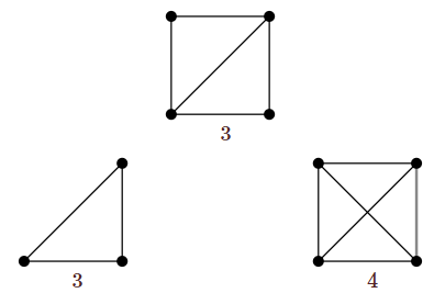
The chromatic number of the graph at the top is \(\min(3,4)=3\). (Of course, this is quite easy to see directly.)

Contributors and Attributions

• Template:ContribGuichard