5.1: Definición y Propiedades

Definición. Vamos\(f\in C_0^s(\mathbb{R}^n)\),\(s=0,1,\ldots\). La función\(\hat{f}\) definida por
\ begin {ecuación}
\ label {four1}
\ anchohat {f} (\ xi) =( 2\ pi) ^ {-n/2}\ int_ {\ mathbb {R} ^n}\ e^ {-i\ xi\ cdot x} f (x)\ dx,
\ end {ecuación}
donde\(\xi\in\mathbb{R}^n\), se llama {\ it transformada de Fourier} de\(f\), y la función\(\widetilde{g}\)
dada por
\ begin {ecuación}
\ label {invfour1}
\ Widetilde {g} (x) =( 2\ pi) ^ {-n/2}\ int_ {\ mathbb {R} ^n}\ e^ {i\ xi\ cdot x} g (\ xi)\ d\ xi
\ end {ecuación}
se llama transformada inversa de Fourier, siempre que
existan las integrales en el lado derecho.

De (\ ref {four1}) se deduce por integración por partes que la diferenciación de una función se cambia a multiplicación de sus transformadas de Fourier, o una operación analítica se convierte en una operación algebraica. Más precisamente, tenemos

Proposición 5.1.

$$
\ sombrero ancho {D^\ alfa f} (\ xi) =i^ {|\ alfa|}\ xi^\ alfa\ sombrero ancho {f} (\ xi),
$$
donde\(|\alpha|\le s\).

La siguiente proposición muestra que la transformada de Fourier de\(f\) disminuye rápidamente para\(|\xi|\to\infty\), siempre y cuando\(f\in C_0^s(\mathbb{R}^n)\). En particular, el lado derecho de (\ ref {invfour1}) existe para\(g:=\hat{f}\) if\(f\in C_0^{n+1}(\mathbb{R}^n)\).

Proposición 5.2. Supongamos\(g\in C_0^s(\mathbb{R}^n)\), entonces hay una constante\(M=M(n,s,g)\) tal que
$$
|\ anchohat {g} (\ xi) |\ le\ frac {M} {(1+|\ xi|) ^s}.
\]

Comprobante. \(\xi=(\xi_1,\ldots,\xi_n)\)Déjese fijar y dejar que\(j\) sea un índice tal que
\(|\xi_j|=\max_k |\xi_k|\). Entonces
$$
|\ xi|=\ left (\ sum_ {k=1} ^n\ xi_k^2\ derecha) ^ {1/2}\ le\ sqrt {n} |\ xi_j|
$$ lo
que implica
\ begin {eqnarray*}
(1+|\ xi|) ^s&=&\ sum_ {k=0} ^s {s\ elige k} |\ xi^k\
&\ le&2^s\ suma_ {k=0} ^sn^ {k/2} |\ xi_j|^k \\
&\ le&2^sn^ {s/2}\ sum_ {|\ alpha|\ le s} |\ xi^\ alpha|.
\ end {eqnarray*}
Esta desigualdad y Proposición 5.1 implican
\ begin {eqnarray*}
(1+|\ xi|) ^s|\ anchohat {g} (\ xi) |&\ le&2^sn^ {s/2}\ sum_ {|\ alpha|\ le s} | (i\ xi) ^\ alpha\ anchohat {g} (\ xi) |\\
&\ le&2^sn^ {s/2}\ sum_ {|\ alpha|\ le s}\ int_ {\ mathbb {R} ^n}\ |D^\ alfa g (x) |\ dx=:M.
\ fin {eqnarray*}

\(\Box\)

La notación inversa transformada de Fourier para (\ ref {invfour1}) se justifica por

Teorema 5.1. \(\widetilde{\widehat{f}}=f\)y\(\widehat{\widetilde{f}}=f\).

Comprobante. Ver\ cite {Yosida}, por ejemplo. Vamos a probar la primera aserción
\ begin {ecuación}
\ label {four2}
(2\ pi) ^ {-n/2}\ int_ {\ mathbb {R} ^n}\ e^ {i\ xi\ cdot x}\ anchohat {f} (\ xi)\ d\ xi=f (x)
\ end {ecuación}
aquí. La prueba de la otra relación se deja como ejercicio. Todas las integrales que aparecen en lo siguiente existen, ver Proposición 5.2 y la elección especial de\(g\).

(i) Fórmula
\ begin {ecuación}
\ etiqueta {cuatro3}
\ int_ {\ mathbb {R} ^n}\ g (\ xi)\ sombrero ancho {f} (\ xi) e^ {ix\ cdot\ xi}\ d\ xi=\ int_ {\ mathbb {R} ^n}\\ sombrero ancho {g} (y) f (x+y)
\ dy\ ecuación final}
sigue por cálculo directo:
\ begin {eqnarray*}
&&\ int_ {\ mathbb {R} ^n}\ g (\ xi)\ izquierda ((2\ pi) ^ {-n/2}\ int_ {\ mathbb {R} ^n}\ e^ {-ix\ cdot y} f (y)\ dy\ derecha) e^ {i x\ cdot\ xi}\ d\ xi\
&&\ qquad =( 2\ pi) ^ {-n/2}\ int_ {\ mathbb {R} ^n}\ izquierda (\ int_ {\ mathbb {R} ^n}\ g (\ xi) e^ {-i\ xi\ cdot (y-x)}\ d\ xi\ derecha) f (y)\ dy\\
&&\ qquad =\ int_ {\ mathbb {R} ^n}\\ sombrero ancho {g} (y-x) f (y)\ dy\\
&&\ qquad=\ int_ {\ mathbb {R} ^n}\\ sombrero ancho {g} (y) f (x+y)\ dy.
\ end {eqnarray*}

(ii) Fórmula
\ begin {ecuación}
\ label {cuatro4}
(2\ pi) ^ {-n/2}\ int_ {\ mathbb {R} ^n}\ e^ {-i y\ cdot\ xi} g (\ varepsilon\ xi)\ d\ xi=\ varepsilon^ {-n}\ sombrero ancho {g} (y/\ varepsilon)
\ end {ecuación}
para cada uno\(\varepsilon>0\) sigue después de la sustitución\(z=\varepsilon\xi\) en el lado izquierdo de (\ ref {four1}).

(iii) Ecuación
\ comenzar {ecuación}
\ etiqueta {cuatro5}
\ int_ {\ mathbb {R} ^n}\ g (\ varepsilon\ xi)\ anchohat {f} (\ xi) e^ {i x\ cdot\ xi}\ d\ xi=\ int_ {\ mathbb {R} ^n}\\ anchohat {g} (y) f (x+\ varepsilon y)\ dy
\ end {ecuación} se
desprende de (\ ref {four3}) y (\ ref {four4} ). Establecer\(G(\xi):=g(\varepsilon\xi)\), entonces (\ ref {four3}) implica
$$
\ int_ {\ mathbb {R} ^n}\ G (\ xi)\ sombrero ancho {f} (\ xi) e^ {i x\ cdot\ xi}\ d\ xi=\ int_ {\ mathbb {R} ^n}\\ sombrero ancho {G} (y) f (x+y)\ dy.
$$
Desde, ver (\ ref {four4}),
\ begin {eqnarray*}
\ anchohat {G} (y) &=& (2\ pi) ^ {-n/2}\ int_ {\ mathbb {R} ^n}\ e^ {-iy\ cdot\ xi} g (\ varepsilon\ xi)\ d\ xi\ &=&\ varepsilon\ xi)\ d\ xi\
&=&\ varepsilon\ xi) psilon^ {-n}\ sombrero ancho {g} (y/\ varepsilon),
\ end {eqnarray*}
llegamos a
\ begin {eqnarray*}
\ int_ {\ mathbb {R} ^n}\ g (\ varepsilon\ xi)\ anchohat {f} (\ xi) &=&\ int_ {\ mathbb {R} ^n}\ varepsilon^ {-n}\ anchohat {g} (y/\ varepsilon) f (x+y)\ dy\\
&=&\ int_ {\ mathbb {R} ^n}\ sombrero ancho {g} (z) f (x+\ varepsilon z)\ dz.
\ end {eqnarray*}
Dejando\(\varepsilon\to 0\), obtenemos
\ begin {ecuación}
\ label {four6}
g (0)\ int_ {\ mathbb {R} ^n}\\ anchohat {f} (\ xi) e^ {i x\ cdot\ xi}\ d\ xi=f (x)\ int_ {\ mathbb {R} ^n}\\ anchohat {g} y ()\ dy.
\ end {ecuación}
Establecer
$$
g (x) :=e^ {-|x|^2/2},
$$
entonces
\ begin {ecuación}
\ label {four7}
\ int_ {\ mathbb {R} ^n}\\ sombrero ancho {g} (y)\ dy =( 2\ pi) ^ {n/2}.
\ end {ecuación}
Ya que\(g(0)=1\), la primera afirmación del Teorema 5.1 se desprende de (\ ref {four6}) y (\ ref {four7}). Queda por mostrar (\ ref {four7}).

iv) Prueba de (\ ref {four7}). Mostraremos
\ begin {eqnarray*}
\ sombrero ancho {g} (y) :&=& (2\ pi) ^ {-n/2}\ int_ {\ mathbb {R} ^n}\ e^ {-|x|^2/2} e^ {-ix\ cdot x}\ dx\\
&=&e^ {-|y|^2/2}.
\ end {eqnarray*}
La prueba de
$$
\ int_ {\ mathbb {R} ^n}\ e^ {-|y|^2/2}\ dy =( 2\ pi) ^ {n/2}
$$
se deja como ejercicio. Desde
$$
-\ izquierda (\ frac {x} {\ sqrt {2}} +i\ frac {y} {\ sqrt {2}}\ derecha)\ cdot\ izquierda (\ frac {x} {\ sqrt {2}} +i\ frac {y} {\ sqrt {2}}\ derecha) =-\ izquierda (\ frac {|x^2} 2} +i x\ cdot y-\ frac {|y|^2} {2}\ derecha)
$$
sigue
\ begin {eqnarray*}
\ int_ {\ mathbb {R} ^n}\ e^ {-|x|^2/2} e^ {-ix\ cdot y}\ dx&=&\ int_ {\ mathbb {R} ^n}\ e^ {-\ eta^2} e^ {-|y|^2/2}\ dx\\
&=&e^ {-|y|y|^2/2}\ int_ {\ mathbb {R} ^n}\ e^ {-\ eta^2}\ dx\\
&=&2^ {n/2} e^ {-|y|^2/2}\ int_ {\ mathbb {R} ^n}\ e^ {-\ eta^2}\ d\ eta
\ end {eqnarray*}
donde
$$
\ eta: =\ frac {x} {\ sqrt {2}} +i\ frac {y} {\ sqrt {2}}.
$$
Considera primero el caso unidimensional. Según el teorema de Cauchy tenemos
$$
\ oint_C\ e^ {-\ eta^2}\ d\ eta=0,
$$
donde la integración es a lo largo de la curva\(C\) que es la unión de cuatro curvas como se indica en la Figura\ ref {fourfig}.

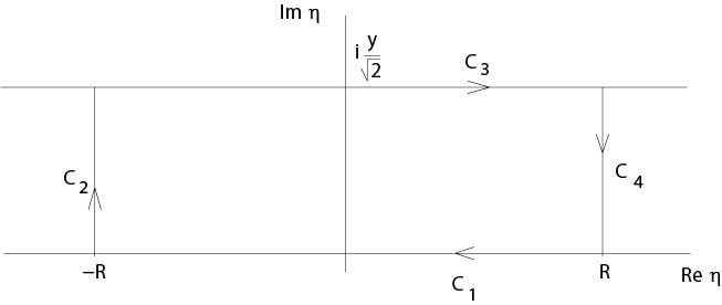
Figura 5.1.1: Prueba de (\ ref {four7})

En consecuencia
$$
\ int_ {C_3}\ e^ {-\ eta^2}\ d\ eta=\ frac {1} {\ sqrt {2}}\ int_ {-R} ^R\ e^ {-x^2/2}\ dx-\ int_ {C_2}\ e^ {-\ eta^2}\ d eta \-\ int_ {C_4}\ e^ {-\ eta^2}\ d\ eta.
$$
Sigue
$$
\ lim_ {R\ a\ infty}\ int_ {C_3}\ e^ {-\ eta^2}\ d\ eta=\ sqrt {\ pi}
$$
desde
$$
\ lim_ {R\ a\ infty}\ int_ {c_k}\ e^ {-\ eta^2}\ d\ eta=0,\ k=2,\ 4.
$$
El caso se\(n>1\) puede reducir al caso unidimensional de la siguiente manera. Set
$$
\ eta=\ frac {x} {\ sqrt {2}} +i\ frac {y} {\ sqrt {2}} =(\ eta_1,\ ldots,\ eta_n),
$$
donde
$$
\ eta_l=\ frac {x_l} {\ sqrt {2}} +i\ frac {y_l} {\ sqrt {2}.
$$
De\(d\eta=d\eta_1\ldots d\eta_l\) y
$$
e^ {-\ eta^2} =e^ {-\ sum_ {l=1} ^n\ eta_l^2} =\ prod_ {l=1} ^ne^ {-\ eta_l^2}
$$
sigue
$$
\ int_ {\ mathbb {R} ^n}\ e^ {-eta^2}\ d\ eta=\ prod_ {l=1} ^n\ int_ {\ gamma_l}\ e^ {-\ eta_l^2}\ d\ eta_l,
$$
donde para fijo\(y\)
$$
\ gamma_l=\ {z\ in {\ mathbb C}:\ z=\ frac {x_l} {\ sqrt {2}} +i\ frac {y_l} {\ sqrt {2}}, -\ infty<x_l<+\ infty\}.
\]

\(\Box\)

Existe una clase útil de funciones para las que existen las integrales en la definición de\(\widehat{f}\) y\(\widetilde{f}\) existen.

Para\(u\in C^\infty(\mathbb{R}^n)\) establecemos
$$
q_ {j, k} (u) :=\ max_ {\ alpha:\ |\ alpha|\ le k}\ left (\ sup_ {\ mathbb {R} ^n}\ left ((1+|x|^2) ^ {j/2} |D^\ alpha u (x) |\ right)\ right).
\]

Definición. La clase Schwartz de funciones que disminuyen rápidamente es
$$
{\ mathcal {S}} (\ mathbb {R} ^n) =\ left\ {u\ in C^\ infty (\ mathbb {R} ^n):\ q_ {j, k} (u) <\ infty\\ mbox {para cualquier}\ j, k\ in {\ mathbb N}\ cup\ {0\}\ derecho\}.
\]

Este espacio es un espacio Frechét.

Proposición 5.3. Asumir\(u\in{\mathcal{S}}(\mathbb{R}^n)\), entonces\(\widehat{u}\) y\(\widetilde{u}\in{\mathcal{S}}(\mathbb{R}^n)\).

Comprobante. Véase [24], Capítulo 1.2, por ejemplo, o un ejercicio.

Colaboradores y Atribuciones

• Template:ContribMiersemann
• Template:ContribMarshall