7.5: Ecuación no homogénea

Aquí consideramos soluciones\(u\in C^2(\Omega)\cap C(\overline{\Omega})\) de
\ begin {eqnarray}
\ label {DI1}
-\ triángulo u&=&f (x)\\\ mbox {in}\\ Omega\
\ etiqueta {DI2}
u&=&0\\\\ mbox {on}\\\ parcial\ Omega,
\ end {eqnarray}
donde \(f\)se da.

Necesitamos el siguiente lema en cuanto a los potenciales de volumen. Suponemos que\(\Omega\) es acotado y suficientemente regular como para que existan todas las siguientes integrales. Véase [6] para las generalizaciones relativas a estos supuestos.

Dejar para\(x\in\mathbb{R}^n\),\(n\ge3\),
$$
V (x) =\ int_\ Omega\ f (y)\ frac {1} {|x-y|^ {n-2}}\ dy
$$
y establecido en el caso bidimensional
$$
V (x) =\ int_\ Omega\ f (y)\ ln\ left (\ frac {1} {|x-y|}\ derecho)\ dy.
$$ Eso
lo recordamos\(\omega_n=|\partial B_1(0)|\).

Lema.
(i) Asumir\(f\in C(\Omega)\). Entonces\(V\in C^1(\mathbb{R}^n)\) y
\ comenzar {eqnarray*}
V_ {x_i} (x) &=&\ int_\ Omega\ f (y)\ frac {\ parcial} {\ parcial} {\ x_i}\ izquierda (\ frac {1} {|x-y|^ {n-2}}\ derecha)\ dy,\\\ mbox {if}\ n\ ge3,\\
V_ {_i} (x) &=&\ int_\ Omega\ f (y)\ frac {\ parcial} {\ parcial} {\ parcial x_i}\ izquierda (\ ln\ izquierda (\ frac {1} {|x-y|}\ derecha)\ derecha)\ dy\\\ mbox {si}\ n=2.
\ end {eqnarray*}
(ii) Si\(f\in C^1(\Omega)\), entonces\(V\in C^2(\Omega)\) y
\ comenzar {eqnarray*}
\ triángulo V&=&- (n-2)\ omega_n f (x),\ x\ in\ Omega,\ n\ ge 3\
\ triángulo V&=&-2\ pi f (x),\ x\ en Omega\,\ n=2.
\ end {eqnarray*}

Comprobante. Para simplificar la presentación, consideramos el caso\(n=3\).
(i) Sigue la primera aseveración ya que podemos cambiar la diferenciación con la integración ya que el integrando diferenciado es débilmente singular, ver un ejercicio.

(ii) Diferenciaremos en\(x\in\Omega\). Dejar\(B_\rho\) ser una bola fija tal que\(x\in B_\rho\),\(\rho\) suficientemente pequeña como para que\(B_\rho\subset\Omega\). Entonces, según (i)
y como tenemos la identidad
$$
\ frac {\ parcial} {\ parcial x_i}\ left (\ frac {1} {|x-y|}\ right) =-\ frac {\ parcial} {\ partial} {\ partial y_i}\ left (\ frac {1} {|x-y|}\ right)
$$ lo
que implica que
$$
f (y)\ frac {\ parcial} {\ parcial x_i}\ izquierda (\ frac {1} {|x-y|}\ derecha) =-\ frac {\ parcial} {\ parcial y_i}\ izquierda (f (y)\ frac {1} {|x-y|}\ derecha) +f_ {y_i} (y)\ frac {1} {|x-y|},
obtenemos
$$
\ begin {eqnarray*}
V_ {x_i} (x) &=&\ int_\ Omega\ f (y)\ frac {\ parcial} {\ parcial x_i}\ izquierda (\ frac {1} {|x-y|}\ derecha)\ dy\
&=&\ int_ {\ Omega\ setmenos B_\ rho}\ f (y)\ frac {\ parcial} {\ parcial} {\ parcial x_i}\ izquierda (\ frac {1} {|x-y|}\ derecha)\ dy+\ int_ {B_\ rho}\ f (y)\ frac {\ parcial} {\ parcial x_i}\ izquierda (\ frac {1} {|x-y|}\ derecha)\ dy\
&=&\ int_ {\ Omega\ setmenos B_\ rho}\ f (y)\ frac {\ parcial} {\ parcial x_i}\ izquierda (\ frac {1} {|x-y|}\ derecha)\ dy\
&&+\ int_ {B_\ rho}\\ izquierda (-\ frac {\ parcial} {\ parcial} {\ parcial y_i}\ izquierda (f (y)\ frac {1} {|x-y|}\ derecha) +f_ {y_i} (y)\ frac ac {1} {|x-y|}\ derecha)\ dy\
&=&\ int_ {\ Omega\ setmenos B_\ rho}\ f (y)\ frac {\ parcial} {\ parcial x_i}\ izquierda (\ frac {1} {|x-y|}\ derecha)\ dy\\
&&&+\ int_ {B_\ rho}\ f_ {y_i} (y)\ frac {1} {|x-y|}\ dy-\ int_ {\ parcial B_\ rho}\ f (y)\ frac {1} {|x-y|} n_i\ ds_y,
\ end {eqnarray*}
donde\(n\) esta el exterior unidad normal a\(\partial B_\rho\). De ello se deduce que la primera y segunda integral está en\(C^1(\Omega)\). La segunda integral también está en\(C^1(\Omega)\) según (i) y desde\(f\in C^1(\Omega)\) por supuesto.

Debido a\(\triangle_x(|x-y|^{-1})=0,\ x\not=y\), sigue
\ begin {eqnarray*}
\ triángulo V&=&\ int_ {B_\ rho}\ suma_ {i=1} ^n f_ {y_i} (y)\ frac {\ parcial} {\ parcial} {\ parcial x_i}\ izquierda (\ frac {1} {|x-y|}\ derecha)\ dy\
&&\ -\ int_ {parcial B_\ rho}\ f (y)\ suma_ {i=1} ^n\ frac {\ parcial} {\ parcial x_i}\ izquierda (\ frac {1} {|x-y|}\ derecha) n_i\ ds_y.
\ end {eqnarray*}
Ahora elegimos para\(B_\rho\) una pelota con el centro en\(x\), entonces
$$
\ triángulo V=I_1+I_2,
$$
donde
\ begin {eqnarray*}
I_1&=&\ int_ {B_\ rho (x)}\\ suma_ {i=1} ^n f_ {y_i} (y)\ frac {y_i-x_i} {|x-y|^3}\ dy\
I_2&=&-\ int_ {\ parcial B_\ rho (x)}\ f (y)\ frac {1} {\ rho^2}\ _y.
\ end {eqnarray*}
Recordamos que\(n\cdot(y-x)=\rho\) si\(y\in\partial B_\rho(x)\). Es\(I_1=O(\rho)\) como\(\rho\to 0\) y para\(I_2\) obtenemos del teorema del valor medio del cálculo integral que para un\(\overline{y}\in\partial B_\rho(x)\)
\ begin {eqnarray*}
I_2&=&-\ frac {1} {\ rho^2} f (\ overline {y})\ int_ {\ parcial B_\ rho (x)}\ ds_y\\
&=&-\ omega_nf (\ overline {y}),
\ end {eqnarray*}
lo que implica que\(\lim_{\rho\to0} I_2=-\omega_nf(x)\).

\(\Box\)

A continuación asumimos que la función de Green existe para el dominio\(\Omega\), que es el caso si\(\Omega\) es una pelota.

Teorema 7.3. Asumir\(f\in C^1(\Omega)\cap C(\overline{\Omega})\). Entonces
$$
u (x) =\ int_\ Omega\ G (x, y) f (y)\ dy
$$
es la solución del problema no homogéneo (\ ref {DI1}), (\ ref {DI2}).

Comprobante. Por simplicidad de la presentación vamos\(n=3\). Mostraremos que
$$
u (x) :=\ int_\ Omega\ G (x, y) f (y)\ dy
$$ es una solución de (7.3.1.1), (7.3.1.2). Desde
$$
G (x, y) =\ frac {1} {4\ pi|x-y|} +\ phi (x, y),
$$
donde\(\phi\) es una función potencial con respecto a\(x\) o\(y\), obtenemos del lema anterior que
\ begin {eqnarray*}
\ triángulo u&=&\ frac {1 } {4\ pi}\ triángulo\ int_\ Omega\ f (y)\ frac {1} {|x-y|}\ dy+\ int_\ Omega\ triangle_x\ phi (x, y) f (y)\ dy\\
&=&-f (x),
\ end {eqnarray*}
donde\(x\in\Omega\). Queda por mostrar que\(u\) logra sus valores límite. Es decir, para fijo\(x_0\in\partial\Omega\) probaremos que
$$
\ lim_ {x\ a x_0,\ x\ in\ Omega} u (x) =0.
$$
Conjunto
$$
u (x) =I_1+I_2,
$$
donde
\ comienza {eqnarray*}
I_1 (x) &=&\ int_ {\ Omega\ setmenos B_\ rho (x_0)}\ G (x, y) f (y)\ dy,\\
I_2 (x) &=&\ int_ {\ Omega\ cap B_\ rho (x_0)}\ G (x, y) f (y)\ dy.
\ end {eqnarray*}
Vamos\(M=\max_{\overline{\Omega}}|f(x)|\). Desde
$$
G (x, y) =\ frac {1} {4\ pi}\ frac {1} {|x-y|} +\ phi (x, y),
$$
obtenemos, si\(x\in B_\rho(x_0)\cap\Omega\),
\ begin {eqnarray*}
|I_2|&\ le&\ frac {M} {4\ pi}\ int_ {\ Omega\ cap B_\ rho (x_0)}\\ frac {dy} {|x-y|} +O (\ rho^2)\\
& amp;\ le&\ frac {M} {4\ pi}\ int_ {B_ {2\ rho (x)}}\\ frac {dy} {|x-y|} +O (\ rho^2)\\
&=&O (\ rho^2)
\ end {eqnarray*}
as\(\rho\to0\). En consecuencia para dado\(\epsilon\) hay\(\rho_0=\rho_0(\epsilon)>0\) tal que
$$
|I_2|<\ frac {\ epsilon} {2}\\\ mbox {para todos}\\ 0<\ rho\ le\ rho_0.
$$
Por cada fijo\(\rho\),\(0<\rho\le\rho_0\), tenemos
$$
\ lim_ {x\ a x_0,\ x\ in\ Omega} I_1 (x) =0
$$
ya que\(G(x_0,y)=0\) si\(y\in\Omega\setminus B_\rho(x_0)\) y\(G(x,y)\) es uniformemente continuo en\(x\in B_{\rho/2}(x_0)\cap\Omega\) y\(y\in\Omega\setminus B_\rho(x_0)\), ver Figura 7.5.1.

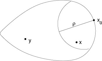
Figura 7.5.1: Prueba de teorema 7.3

\(\Box\)

OBSERVACIÓN. Para la prueba de (ii) en el lema anterior es suficiente asumir que\(f\) es H\ "mayor continuo. Más precisamente, vamos
\(f\in C^{\lambda}(\Omega)\)\(0<\lambda<1\), entonces\(V\in C^{2,\lambda}(\Omega)\), ver por ejemplo [9].

Colaboradores y Atribuciones

• Template:ContribMiersemann
• Template:ContribMarshall