4.5: Modelos de deterioro artificial de redes neuronales
- Page ID
- 59669

Las redes neuronales artificiales pueden servir como alternativa a los modelos de regresión o deterioro de Markov. Se basan en una analogía a cómo se comportan los cerebros biológicos simples en la transmisión de señales entre células neuronales individuales. Se originaron en el trabajo sobre inteligencia artificial y aprendizaje automático.
La Figura 4.5.1 ilustra una red neuronal. Los insumos pueden ser valores de índice de condición, edad o efectos climáticos. Los resultados pueden ser probabilidades de transición a condiciones particulares en el transcurso de un año. La Figura 4.5.1 ilustra el procesamiento de señal que estaría ocurriendo dentro de cada una de las neuronas artificiales (representadas como círculos en la Figura 4.5.1). Las señales de entrada son ponderadas, combinadas y transformadas en una activación de salida.
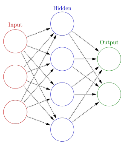
Figura\(\PageIndex{1}\): Illustration of a Neural Network with Input, Hidden and Output Stages. Source: By Glosser.ca - Own work, Derivative of File:Artificial neural network.svg, CC BY-SA 3.0, https://commons.wikimedia.org/w/inde...curid=24913461.
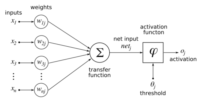
Artificial neural networks are typically ‘trained’ with a learning set. For a deterioration model, inputs might consist of conditions (and other relevant factors) in the base year and the training outputs would be the observed conditions in the following year. Training consists of altering parameters (such as the weights in Figure 4.5.2) to best reproduce the results observed in the training set.
Artificial neural networks are not frequently used for component deterioration modelling. One drawback to their use is the ‘black box’ nature of the results where the various weights and activation functions are difficult to interpret (or even obtain). Also, artificial neural networks typically have many more parameters than other types of models, requiring more data to be robust.
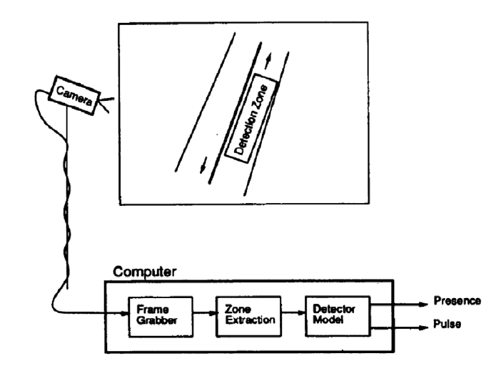
Infrastructure managers are more likely to encounter artificial neural networks in conjunction with sensor interpretation. For example, artificial neural networks can be used to identify vehicles or pavement distress from video inputs. Figure 4.5.3 illustrates a video-based system for vehicle identification. A frame from the camera is divided into a two dimensional set of tiles within a pre-defined detection zone and the color and brightness of the pixels within each tile are input to an artificial neural network vehicle detector model. A training set of images with and without vehicles is used to adjust parameters in the detector model. In turn, traffic identification of this type can be used in a deterioration model for pavement condition.
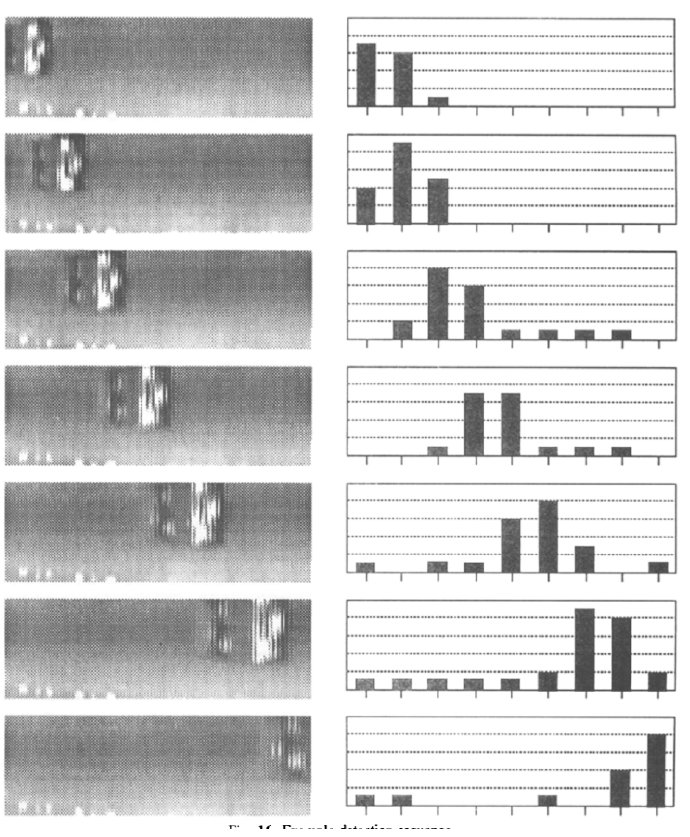
A detection sequence for the video vehicle identification is illustrated in Figure 4.5.4. As the vehicle moves through the detection zone, counting output is activated for each part of the zone.