
14.1: Introducción a los vectores
- Page ID
- 69861
\( \newcommand{\vecs}[1]{\overset { \scriptstyle \rightharpoonup} {\mathbf{#1}} } \)
\( \newcommand{\vecd}[1]{\overset{-\!-\!\rightharpoonup}{\vphantom{a}\smash {#1}}} \)
\( \newcommand{\id}{\mathrm{id}}\) \( \newcommand{\Span}{\mathrm{span}}\)
( \newcommand{\kernel}{\mathrm{null}\,}\) \( \newcommand{\range}{\mathrm{range}\,}\)
\( \newcommand{\RealPart}{\mathrm{Re}}\) \( \newcommand{\ImaginaryPart}{\mathrm{Im}}\)
\( \newcommand{\Argument}{\mathrm{Arg}}\) \( \newcommand{\norm}[1]{\| #1 \|}\)
\( \newcommand{\inner}[2]{\langle #1, #2 \rangle}\)
\( \newcommand{\Span}{\mathrm{span}}\)
\( \newcommand{\id}{\mathrm{id}}\)
\( \newcommand{\Span}{\mathrm{span}}\)
\( \newcommand{\kernel}{\mathrm{null}\,}\)
\( \newcommand{\range}{\mathrm{range}\,}\)
\( \newcommand{\RealPart}{\mathrm{Re}}\)
\( \newcommand{\ImaginaryPart}{\mathrm{Im}}\)
\( \newcommand{\Argument}{\mathrm{Arg}}\)
\( \newcommand{\norm}[1]{\| #1 \|}\)
\( \newcommand{\inner}[2]{\langle #1, #2 \rangle}\)
\( \newcommand{\Span}{\mathrm{span}}\) \( \newcommand{\AA}{\unicode[.8,0]{x212B}}\)
\( \newcommand{\vectorA}[1]{\vec{#1}} % arrow\)
\( \newcommand{\vectorAt}[1]{\vec{\text{#1}}} % arrow\)
\( \newcommand{\vectorB}[1]{\overset { \scriptstyle \rightharpoonup} {\mathbf{#1}} } \)
\( \newcommand{\vectorC}[1]{\textbf{#1}} \)
\( \newcommand{\vectorD}[1]{\overrightarrow{#1}} \)
\( \newcommand{\vectorDt}[1]{\overrightarrow{\text{#1}}} \)
\( \newcommand{\vectE}[1]{\overset{-\!-\!\rightharpoonup}{\vphantom{a}\smash{\mathbf {#1}}}} \)
\( \newcommand{\vecs}[1]{\overset { \scriptstyle \rightharpoonup} {\mathbf{#1}} } \)
\( \newcommand{\vecd}[1]{\overset{-\!-\!\rightharpoonup}{\vphantom{a}\smash {#1}}} \)
\(\newcommand{\avec}{\mathbf a}\) \(\newcommand{\bvec}{\mathbf b}\) \(\newcommand{\cvec}{\mathbf c}\) \(\newcommand{\dvec}{\mathbf d}\) \(\newcommand{\dtil}{\widetilde{\mathbf d}}\) \(\newcommand{\evec}{\mathbf e}\) \(\newcommand{\fvec}{\mathbf f}\) \(\newcommand{\nvec}{\mathbf n}\) \(\newcommand{\pvec}{\mathbf p}\) \(\newcommand{\qvec}{\mathbf q}\) \(\newcommand{\svec}{\mathbf s}\) \(\newcommand{\tvec}{\mathbf t}\) \(\newcommand{\uvec}{\mathbf u}\) \(\newcommand{\vvec}{\mathbf v}\) \(\newcommand{\wvec}{\mathbf w}\) \(\newcommand{\xvec}{\mathbf x}\) \(\newcommand{\yvec}{\mathbf y}\) \(\newcommand{\zvec}{\mathbf z}\) \(\newcommand{\rvec}{\mathbf r}\) \(\newcommand{\mvec}{\mathbf m}\) \(\newcommand{\zerovec}{\mathbf 0}\) \(\newcommand{\onevec}{\mathbf 1}\) \(\newcommand{\real}{\mathbb R}\) \(\newcommand{\twovec}[2]{\left[\begin{array}{r}#1 \\ #2 \end{array}\right]}\) \(\newcommand{\ctwovec}[2]{\left[\begin{array}{c}#1 \\ #2 \end{array}\right]}\) \(\newcommand{\threevec}[3]{\left[\begin{array}{r}#1 \\ #2 \\ #3 \end{array}\right]}\) \(\newcommand{\cthreevec}[3]{\left[\begin{array}{c}#1 \\ #2 \\ #3 \end{array}\right]}\) \(\newcommand{\fourvec}[4]{\left[\begin{array}{r}#1 \\ #2 \\ #3 \\ #4 \end{array}\right]}\) \(\newcommand{\cfourvec}[4]{\left[\begin{array}{c}#1 \\ #2 \\ #3 \\ #4 \end{array}\right]}\) \(\newcommand{\fivevec}[5]{\left[\begin{array}{r}#1 \\ #2 \\ #3 \\ #4 \\ #5 \\ \end{array}\right]}\) \(\newcommand{\cfivevec}[5]{\left[\begin{array}{c}#1 \\ #2 \\ #3 \\ #4 \\ #5 \\ \end{array}\right]}\) \(\newcommand{\mattwo}[4]{\left[\begin{array}{rr}#1 \amp #2 \\ #3 \amp #4 \\ \end{array}\right]}\) \(\newcommand{\laspan}[1]{\text{Span}\{#1\}}\) \(\newcommand{\bcal}{\cal B}\) \(\newcommand{\ccal}{\cal C}\) \(\newcommand{\scal}{\cal S}\) \(\newcommand{\wcal}{\cal W}\) \(\newcommand{\ecal}{\cal E}\) \(\newcommand{\coords}[2]{\left\{#1\right\}_{#2}}\) \(\newcommand{\gray}[1]{\color{gray}{#1}}\) \(\newcommand{\lgray}[1]{\color{lightgray}{#1}}\) \(\newcommand{\rank}{\operatorname{rank}}\) \(\newcommand{\row}{\text{Row}}\) \(\newcommand{\col}{\text{Col}}\) \(\renewcommand{\row}{\text{Row}}\) \(\newcommand{\nul}{\text{Nul}}\) \(\newcommand{\var}{\text{Var}}\) \(\newcommand{\corr}{\text{corr}}\) \(\newcommand{\len}[1]{\left|#1\right|}\) \(\newcommand{\bbar}{\overline{\bvec}}\) \(\newcommand{\bhat}{\widehat{\bvec}}\) \(\newcommand{\bperp}{\bvec^\perp}\) \(\newcommand{\xhat}{\widehat{\xvec}}\) \(\newcommand{\vhat}{\widehat{\vvec}}\) \(\newcommand{\uhat}{\widehat{\uvec}}\) \(\newcommand{\what}{\widehat{\wvec}}\) \(\newcommand{\Sighat}{\widehat{\Sigma}}\) \(\newcommand{\lt}{<}\) \(\newcommand{\gt}{>}\) \(\newcommand{\amp}{&}\) \(\definecolor{fillinmathshade}{gray}{0.9}\)En este capítulo revisaremos algunos conceptos que probablemente conozcas de tus cursos de física. Este capítulo no pretende cubrir el tema de manera integral, sino que toca algunos conceptos que usarás en tus clases de química física.
Un vector es una cantidad que tiene tanto una magnitud como una dirección, y como tales se utilizan para especificar la posición, velocidad e impulso de una partícula, o para especificar una fuerza. Los vectores generalmente se denotan con símbolos en negritas (por ejemplo\(\mathbf{u}\)) o con una flecha encima del símbolo (por ejemplo\(\vec{u}\)). Una tilde colocada encima o debajo del nombre del vector también se usa comúnmente en taquigrafía (\(\widetilde{u}\),\(\underset{\sim}{u}\)).
Si multiplicamos un número\(a\) por un vector\(\mathbf{v}\), obtenemos un nuevo vector que es paralelo al original pero con una longitud que es\(a\) por la longitud de\(\mathbf{v}\). Si\(a\) es\(a\mathbf{v}\) puntos negativos en la dirección opuesta a la\(\mathbf{v}\). Podemos expresar cualquier vector en términos de los llamados vectores unitarios. Estos vectores, los cuales son designados\(\hat{\mathbf{i}}\),\(\hat{\mathbf{j}}\) y\(\hat{\mathbf{k}}\), tienen unidad de longitud y punto a lo largo del positivo\(x, y\) y\(z\) eje del sistema de coordenadas cartesianas (Figura\(\PageIndex{1}\)). El símbolo\(\hat{\mathbf{i}}\) se lee “i-hat”. Los sombreros se utilizan para denotar que un vector tiene longitud unitaria.
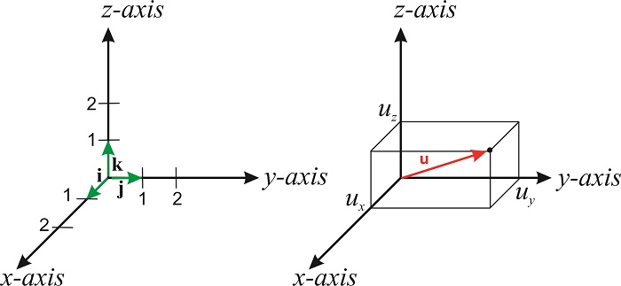
La longitud de\(\mathbf{u}\) es su magnitud (o módulo), y generalmente se denota por\(u\):
\[\label{eq:vectors1} u=|u|=(u_x^2+u_y^2+u_z^2)^{1/2}\]
Si tenemos dos vectores\(\mathbf{u}=u_x\hat{\mathbf{i}}+u_y \hat{\mathbf{j}}+u_z \hat{\mathbf{k}}\) y\(\mathbf{v}=v_x \hat{\mathbf{i}}+v_y \hat{\mathbf{j}}+v_z \hat{\mathbf{k}}\), podemos agregarlos para obtener
\[\mathbf{u}+\mathbf{v}=(u_x+v_x)\hat{\mathbf{i}}+(u_y+v_y)\hat{\mathbf{j}}+(u_z+v_z)\hat{\mathbf{k}} \nonumber\]
o restarlos para obtener:
\[\mathbf{u}-\mathbf{v}=(u_x-v_x)\hat{\mathbf{i}}+(u_y-v_y)\hat{\mathbf{j}}+(u_z-v_z)\hat{\mathbf{k}} \nonumber\]
Cuando se trata de multiplicar, podemos realizar el producto de dos vectores de dos maneras distintas. El primero, que da como resultado un escalar (un número), se denomina producto escalar o producto punto. El segundo, que da como resultado un vector, se llama el producto vector (o cruz). Ambas son operaciones importantes en la química física.