3.6: Trazado MOS I-V

Ahora utilizamos dos de las ecuaciones (3.5.6 y 3.5.10) que encontramos en la discusión sobre Regímenes MOS para calcular un conjunto de\(V_{\text{d sat}}\) y\(I_{\text{d sat}}\) valores para diversos valores de\(V_{\text{gs}}\). (Tenga en cuenta que\(V_{\text{gs}}\) debe ser mayor que\(V_{T}\) para que las dos ecuaciones sean válidas.) Cuando obtenemos los números, construimos una mesita.

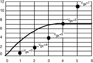
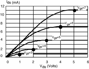
Una vez que tenemos los números (Tabla\(\PageIndex{1}\), luego dibujamos un trozo de papel cuadriculado con la escala adecuada, y trazamos los puntos en él. Una vez determinados los\(\left(I_{\text{d sat}}, \ V_{\text{d sat}}\right)\) puntos, es fácil de esbozar en el\(I\text{-}V\) comportamiento. Simplemente dibujas una curva desde el origen hasta cualquier punto dado, teniéndola “pico hacia fuera” justo en el punto, y luego dibujas una línea recta en\(I_{\text{d sat}}\) para terminar las cosas. Una de esas curvas se muestra en la Figura\(\PageIndex{2}\). Y luego finalmente en Figura\(\PageIndex{3}\) están todos esbozados en. Tus curvas probablemente no serán exactamente correctas pero serán lo suficientemente buenas para muchas aplicaciones.

Tabla\(\PageIndex{1}\): Resultados del cálculo\(V_{\text{d sat}}\) y\(I_{\text{d sat}}\)

\(V_{\text{gs}}\)	\(V_{\text{d sat}} \ (\mathrm{V})\)	\(I_{\text{d sat}} \ (\mathrm{mA})\)
\ (V_ {\ texto {gs}}\) ">\(3\)	\ (V_ {\ texto {d sat}}\ (\ mathrm {V})\) ">\(1\)	\ (I_ {\ texto {d sat}}\ (\ mathrm {mA})\) ">\(0.44\)
\ (V_ {\ texto {gs}}\) ">\(4\)	\ (V_ {\ texto {d sat}}\ (\ mathrm {V})\) ">\(2\)	\ (I_ {\ texto {d sat}}\ (\ mathrm {mA})\) ">\(1.76\)
\ (V_ {\ texto {gs}}\) ">\(5\)	\ (V_ {\ texto {d sat}}\ (\ mathrm {V})\) ">\(3\)	\ (I_ {\ texto {d sat}}\ (\ mathrm {mA})\) ">\(3.96\)
\ (V_ {\ texto {gs}}\) ">\(6\)	\ (V_ {\ texto {d sat}}\ (\ mathrm {V})\) ">\(4\)	\ (I_ {\ texto {d sat}}\ (\ mathrm {mA})\) ">\(7.04\)
\ (V_ {\ texto {gs}}\) ">\(7\)	\ (V_ {\ texto {d sat}}\ (\ mathrm {V})\) ">\(5\)	\ (I_ {\ texto {d sat}}\ (\ mathrm {mA})\) ">\(11\)

Figura\(\PageIndex{1}\): Trazado\(I_{\text{d sat}}\) y\(V_{\text{d sat}}\).

Figura\(\PageIndex{2}\): Esbozo en una de las\(I\text{-}V\) curvas.

Figura\(\PageIndex{3}\): El conjunto completo de curvas.

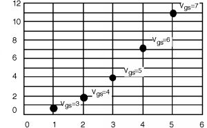
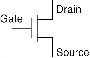
Existe una manera particularmente fácil de medir por\(k\) y\(V_{T}\) para un MOSFET. Primero introduzcamos el símbolo esquemático para el MOSFET; parece Figura\(\PageIndex{4}\). Tomemos un MOSFET y lo conectemos como se muestra en la Figura\(\PageIndex{5}\).

Figura\(\PageIndex{4}\): Símbolo esquemático para un MOSFET

Figura\(\PageIndex{5}\): Circuito para encontrar\(V_{T}\) y\(k\)

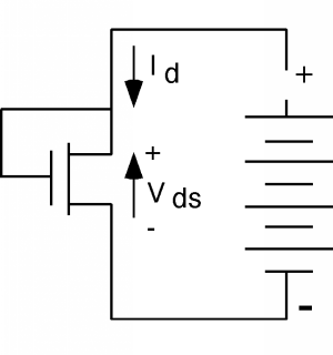
Dado que la puerta de este transistor está conectada al desagüe, no cabe duda de que\(V_{\text{gs}} - V_{\text{ds}}\) es menor que\(V_{T}\). De hecho, ya que\(V_{\text{gs}} = V_{\text{ds}}\), su diferencia es cero. Así, para cualquier valor de\(V_{\text{ds}}\), este transistor está operando en su condición saturada. Ya que\(V_{\text{gs}} = V_{\text{ds}}\), podemos reescribir una ecuación anterior derivada de la sección sobre regímenes MOS como\[I_{d} = \frac{k}{2} \left(V_{\text{ds}} - V_{T}\right)^{2}\]

Ahora tomemos la raíz cuadrada de ambos lados:\[\sqrt{I_{d}} = \sqrt{\frac{k}{2}} \left(V_{\text{ds}} - V_{T}\right)\]

Entonces, si hacemos una trama de\(\sqrt{I_{d}}\) en función de\(V_{\text{ds}}\), deberíamos obtener una línea recta, con una pendiente de\(\sqrt{\frac{k}{2}}\) y una\(x\) -intercepción de\(V_{T}\).

Figura\(\PageIndex{6}\): Obtención\(V_{T}\) y\(k\)

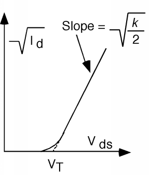
Debido a la no idealidad esperada, la curva no va hasta el final\(V_{T}\), sino que se desvía un poco cerca del fondo. Sin embargo, una simple extrapolación lineal de la parte recta de la gráfica produce un valor inequívoco para el voltaje umbral\(V_{T}\).