
1.8:1.8 Ceros e Intercepciones de Funciones
- Page ID
- 107352
\( \newcommand{\vecs}[1]{\overset { \scriptstyle \rightharpoonup} {\mathbf{#1}} } \)
\( \newcommand{\vecd}[1]{\overset{-\!-\!\rightharpoonup}{\vphantom{a}\smash {#1}}} \)
\( \newcommand{\dsum}{\displaystyle\sum\limits} \)
\( \newcommand{\dint}{\displaystyle\int\limits} \)
\( \newcommand{\dlim}{\displaystyle\lim\limits} \)
\( \newcommand{\id}{\mathrm{id}}\) \( \newcommand{\Span}{\mathrm{span}}\)
( \newcommand{\kernel}{\mathrm{null}\,}\) \( \newcommand{\range}{\mathrm{range}\,}\)
\( \newcommand{\RealPart}{\mathrm{Re}}\) \( \newcommand{\ImaginaryPart}{\mathrm{Im}}\)
\( \newcommand{\Argument}{\mathrm{Arg}}\) \( \newcommand{\norm}[1]{\| #1 \|}\)
\( \newcommand{\inner}[2]{\langle #1, #2 \rangle}\)
\( \newcommand{\Span}{\mathrm{span}}\)
\( \newcommand{\id}{\mathrm{id}}\)
\( \newcommand{\Span}{\mathrm{span}}\)
\( \newcommand{\kernel}{\mathrm{null}\,}\)
\( \newcommand{\range}{\mathrm{range}\,}\)
\( \newcommand{\RealPart}{\mathrm{Re}}\)
\( \newcommand{\ImaginaryPart}{\mathrm{Im}}\)
\( \newcommand{\Argument}{\mathrm{Arg}}\)
\( \newcommand{\norm}[1]{\| #1 \|}\)
\( \newcommand{\inner}[2]{\langle #1, #2 \rangle}\)
\( \newcommand{\Span}{\mathrm{span}}\) \( \newcommand{\AA}{\unicode[.8,0]{x212B}}\)
\( \newcommand{\vectorA}[1]{\vec{#1}} % arrow\)
\( \newcommand{\vectorAt}[1]{\vec{\text{#1}}} % arrow\)
\( \newcommand{\vectorB}[1]{\overset { \scriptstyle \rightharpoonup} {\mathbf{#1}} } \)
\( \newcommand{\vectorC}[1]{\textbf{#1}} \)
\( \newcommand{\vectorD}[1]{\overrightarrow{#1}} \)
\( \newcommand{\vectorDt}[1]{\overrightarrow{\text{#1}}} \)
\( \newcommand{\vectE}[1]{\overset{-\!-\!\rightharpoonup}{\vphantom{a}\smash{\mathbf {#1}}}} \)
\( \newcommand{\vecs}[1]{\overset { \scriptstyle \rightharpoonup} {\mathbf{#1}} } \)
\(\newcommand{\longvect}{\overrightarrow}\)
\( \newcommand{\vecd}[1]{\overset{-\!-\!\rightharpoonup}{\vphantom{a}\smash {#1}}} \)
\(\newcommand{\avec}{\mathbf a}\) \(\newcommand{\bvec}{\mathbf b}\) \(\newcommand{\cvec}{\mathbf c}\) \(\newcommand{\dvec}{\mathbf d}\) \(\newcommand{\dtil}{\widetilde{\mathbf d}}\) \(\newcommand{\evec}{\mathbf e}\) \(\newcommand{\fvec}{\mathbf f}\) \(\newcommand{\nvec}{\mathbf n}\) \(\newcommand{\pvec}{\mathbf p}\) \(\newcommand{\qvec}{\mathbf q}\) \(\newcommand{\svec}{\mathbf s}\) \(\newcommand{\tvec}{\mathbf t}\) \(\newcommand{\uvec}{\mathbf u}\) \(\newcommand{\vvec}{\mathbf v}\) \(\newcommand{\wvec}{\mathbf w}\) \(\newcommand{\xvec}{\mathbf x}\) \(\newcommand{\yvec}{\mathbf y}\) \(\newcommand{\zvec}{\mathbf z}\) \(\newcommand{\rvec}{\mathbf r}\) \(\newcommand{\mvec}{\mathbf m}\) \(\newcommand{\zerovec}{\mathbf 0}\) \(\newcommand{\onevec}{\mathbf 1}\) \(\newcommand{\real}{\mathbb R}\) \(\newcommand{\twovec}[2]{\left[\begin{array}{r}#1 \\ #2 \end{array}\right]}\) \(\newcommand{\ctwovec}[2]{\left[\begin{array}{c}#1 \\ #2 \end{array}\right]}\) \(\newcommand{\threevec}[3]{\left[\begin{array}{r}#1 \\ #2 \\ #3 \end{array}\right]}\) \(\newcommand{\cthreevec}[3]{\left[\begin{array}{c}#1 \\ #2 \\ #3 \end{array}\right]}\) \(\newcommand{\fourvec}[4]{\left[\begin{array}{r}#1 \\ #2 \\ #3 \\ #4 \end{array}\right]}\) \(\newcommand{\cfourvec}[4]{\left[\begin{array}{c}#1 \\ #2 \\ #3 \\ #4 \end{array}\right]}\) \(\newcommand{\fivevec}[5]{\left[\begin{array}{r}#1 \\ #2 \\ #3 \\ #4 \\ #5 \\ \end{array}\right]}\) \(\newcommand{\cfivevec}[5]{\left[\begin{array}{c}#1 \\ #2 \\ #3 \\ #4 \\ #5 \\ \end{array}\right]}\) \(\newcommand{\mattwo}[4]{\left[\begin{array}{rr}#1 \amp #2 \\ #3 \amp #4 \\ \end{array}\right]}\) \(\newcommand{\laspan}[1]{\text{Span}\{#1\}}\) \(\newcommand{\bcal}{\cal B}\) \(\newcommand{\ccal}{\cal C}\) \(\newcommand{\scal}{\cal S}\) \(\newcommand{\wcal}{\cal W}\) \(\newcommand{\ecal}{\cal E}\) \(\newcommand{\coords}[2]{\left\{#1\right\}_{#2}}\) \(\newcommand{\gray}[1]{\color{gray}{#1}}\) \(\newcommand{\lgray}[1]{\color{lightgray}{#1}}\) \(\newcommand{\rank}{\operatorname{rank}}\) \(\newcommand{\row}{\text{Row}}\) \(\newcommand{\col}{\text{Col}}\) \(\renewcommand{\row}{\text{Row}}\) \(\newcommand{\nul}{\text{Nul}}\) \(\newcommand{\var}{\text{Var}}\) \(\newcommand{\corr}{\text{corr}}\) \(\newcommand{\len}[1]{\left|#1\right|}\) \(\newcommand{\bbar}{\overline{\bvec}}\) \(\newcommand{\bhat}{\widehat{\bvec}}\) \(\newcommand{\bperp}{\bvec^\perp}\) \(\newcommand{\xhat}{\widehat{\xvec}}\) \(\newcommand{\vhat}{\widehat{\vvec}}\) \(\newcommand{\uhat}{\widehat{\uvec}}\) \(\newcommand{\what}{\widehat{\wvec}}\) \(\newcommand{\Sighat}{\widehat{\Sigma}}\) \(\newcommand{\lt}{<}\) \(\newcommand{\gt}{>}\) \(\newcommand{\amp}{&}\) \(\definecolor{fillinmathshade}{gray}{0.9}\)Una intercepción en matemáticas es donde una función cruza el\(y\) eje\(x\) o. ¿Cuáles son
las intercepciones de esta función?
Intercepciones X e Y
El primer tipo de intercepción que puede haber aprendido es la\(y\) -intercepción cuando aprendió la forma de intercepción de pendiente de una línea:\(y=m x+b\). A\(y\) -intercept es el punto único donde una función cruza el\(y\) eje. Se puede encontrar algebraicamente estableciendo\(x=0\) y resolviendo para\(y\).
\(x\)-intercepciones son donde las funciones cruzan el\(x\) eje y donde la altura de la función es cero. También se les llama raíces, soluciones y ceros de una función. Se encuentran algebraicamente estableciendo\(y=0\) y resolviendo para\(x\). Vea los videos a continuación para practicar:
Ejemplos
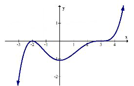
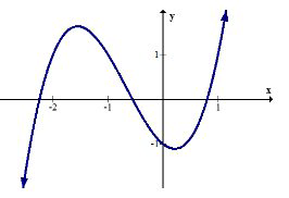
Anteriormente, se le preguntó cuáles son las intercepciones de la gráfica a continuación.
Gráficamente la función tiene ceros en -2 y 3 con una\(y\) intercepción aproximadamente\(-1.1 .\)
Nota: Para que una función pase la prueba de línea vertical, solo debe tener una\(y\) -intercepción, pero puede tener múltiples\(x\) -intercepciones.
Cuáles son los ceros e\(y\) -intercepciones de la parábola\(y=x^{2}-2 x-3 ?\)
Usando una gráfica:
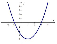
Los ceros están en (-1,0) y (3,0). El\(y\) -intercepto está en (0, -3).
Usando Álgebra:
Sustituye 0 por\(y\) para encontrar ceros.
\(0=x^{2}-2 x-3=(x-3)(x+1)\)
\(y=0, x=3,-1\)
Sustituye 0 por\(x\) para encontrar la\(y\) -intercepción.
\(y=(0)^{2}-2(0)-3=-3\)
\(x=0, y=-3\)
Identificar los ceros e\(y\) intercepciones para la función sinusoidal.
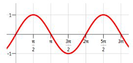
El\(y\) -intercepto es (0,0). Hay cuatro ceros visibles en esta parte de la gráfica. Una cosa que sabes de la gráfica sinusoidal es que es periódica y se repite para siempre en ambas direcciones. Para capturar cada\(x\) -intercepción, debes identificar un patrón en lugar de intentar escribir cada uno.
Las\(x\) intercepciones visibles son\(0, \pi, 2 \pi, 3 \pi\). El patrón es que hay una\(x\) -intercepción cada múltiplo de\(\pi\) incluyendo múltiplos negativos. Para describir todos estos valores debes escribir:
Los\(x\) -intercepts son\(\pm n \pi\) donde\(n\) es un entero\(\{0,\pm 1,\pm 2, \ldots\}\).
Identificar las intercepciones y ceros de la función:\(f(x)=\frac{1}{100}(x-3)^{3}(x+2)^{2}\)
Para encontrar la\(y\) -intercepción, sustituya o por\(x\):
\(y=\frac{1}{100}(0-3)^{3}(0+2)^{2}=\frac{1}{100}(-27)(4)=-\frac{108}{100}=-1.08\)
Para encontrar las\(x\) -intercepciones, sustituya 0 por\(y\):
\(0=\frac{1}{100}(x-3)^{3}(x+2)^{2}\)
\(x=3,-2\)
Así, la\(y\) -intercepción es (0, -1.08) y las\(x\) -intercepciones son (3,0) y (-2,0)
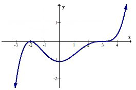
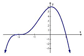
Determinar gráficamente las intercepciones de la siguiente función.
El\(y\) -intercepto es aproximadamente (0, -1). Las\(x\) -intercepciones son aproximadamente (-2.3,0), (-0.4,0) y\((0.7,0) .\) Al encontrar valores gráficamente, las respuestas son siempre aproximadas. Las respuestas exactas deben encontrarse analíticamente.
Revisar
1. Determinar los ceros y\(y\) -interceptar la siguiente función usando álgebra:
\(f(x)=(x+1)^{3}(x-4)\)
2. Determinar las raíces y\(y\) -interceptar la siguiente función usando álgebra o una gráfica:
3. Determine gráficamente las intercepciones de la siguiente función:
Encuentra las intercepciones para cada una de las siguientes funciones.
4. \(y=x^{2}\)
5. \(y=x^{3}\)
6. \(y=\ln (x)\)
7. \(y=\frac{1}{x}\)
8. \(y=e^{x}\)
9. \(y=\sqrt{x}\)
10. ¿Hay alguna función sin una\(y\) intercepción? Explicar.
11. ¿Hay alguna función sin una\(x\) intercepción? Explicar.
12. Explique por qué tiene sentido que una\(x\) -intercepción de una función también se llame
“cero” de la función.
Determinar las intercepciones de las siguientes funciones utilizando álgebra o una gráfica.
13. \(h(x)=x^{3}-6 x^{2}+3 x+10\)
14. \(j(x)=x^{2}-6 x-7\)
15. \(k(x)=4 x^{4}-20 x^{3}-3 x^{2}+14 x+5\)