7.4: Trazando la distribución de una sola variable
- Page ID
- 150796

\( \newcommand{\vecs}[1]{\overset { \scriptstyle \rightharpoonup} {\mathbf{#1}} } \)
\( \newcommand{\vecd}[1]{\overset{-\!-\!\rightharpoonup}{\vphantom{a}\smash {#1}}} \)
\( \newcommand{\id}{\mathrm{id}}\) \( \newcommand{\Span}{\mathrm{span}}\)
( \newcommand{\kernel}{\mathrm{null}\,}\) \( \newcommand{\range}{\mathrm{range}\,}\)
\( \newcommand{\RealPart}{\mathrm{Re}}\) \( \newcommand{\ImaginaryPart}{\mathrm{Im}}\)
\( \newcommand{\Argument}{\mathrm{Arg}}\) \( \newcommand{\norm}[1]{\| #1 \|}\)
\( \newcommand{\inner}[2]{\langle #1, #2 \rangle}\)
\( \newcommand{\Span}{\mathrm{span}}\)
\( \newcommand{\id}{\mathrm{id}}\)
\( \newcommand{\Span}{\mathrm{span}}\)
\( \newcommand{\kernel}{\mathrm{null}\,}\)
\( \newcommand{\range}{\mathrm{range}\,}\)
\( \newcommand{\RealPart}{\mathrm{Re}}\)
\( \newcommand{\ImaginaryPart}{\mathrm{Im}}\)
\( \newcommand{\Argument}{\mathrm{Arg}}\)
\( \newcommand{\norm}[1]{\| #1 \|}\)
\( \newcommand{\inner}[2]{\langle #1, #2 \rangle}\)
\( \newcommand{\Span}{\mathrm{span}}\) \( \newcommand{\AA}{\unicode[.8,0]{x212B}}\)
\( \newcommand{\vectorA}[1]{\vec{#1}} % arrow\)
\( \newcommand{\vectorAt}[1]{\vec{\text{#1}}} % arrow\)
\( \newcommand{\vectorB}[1]{\overset { \scriptstyle \rightharpoonup} {\mathbf{#1}} } \)
\( \newcommand{\vectorC}[1]{\textbf{#1}} \)
\( \newcommand{\vectorD}[1]{\overrightarrow{#1}} \)
\( \newcommand{\vectorDt}[1]{\overrightarrow{\text{#1}}} \)
\( \newcommand{\vectE}[1]{\overset{-\!-\!\rightharpoonup}{\vphantom{a}\smash{\mathbf {#1}}}} \)
\( \newcommand{\vecs}[1]{\overset { \scriptstyle \rightharpoonup} {\mathbf{#1}} } \)
\( \newcommand{\vecd}[1]{\overset{-\!-\!\rightharpoonup}{\vphantom{a}\smash {#1}}} \)
¿Cómo eliges qué geometría usar? ggplot le permite elegir entre una serie de geometrías. Esta elección determinará qué tipo de parcela creas. Utilizaremos el conjunto de datos mpg incorporado, que contiene datos de eficiencia de combustible para varios autos diferentes.
7.4.1 Histograma
El histograma muestra la distribución ogerall de los datos. Aquí usamos la función nClass.fd para calcular el tamaño óptimo de bin.
ggplot(mpg, aes(hwy)) +
  geom_histogram(bins = nclass.FD(mpg$hwy)) +
xlab('Highway mileage') 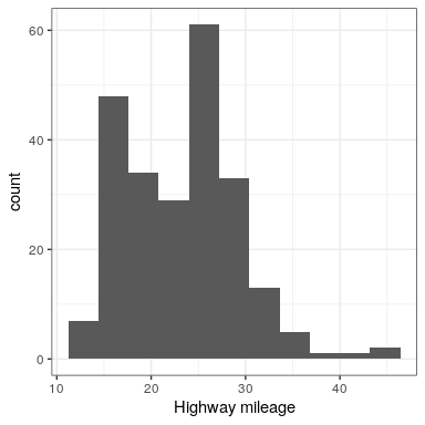
En lugar de crear contenedores discretos, podemos observar la densidad relativa continuamente.
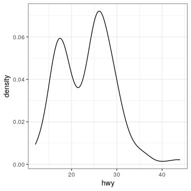
7.4.2 Parcela de densidad
ggplot(mpg, aes(hwy)) +
  geom_density() +
xlab('Highway mileage') 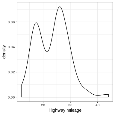
Una nota sobre los valores predeterminados: La estadística predeterminada (o “stat”) subyacente a geom_density se llama “densidad”, lo que no es sorprendente. La estadística predeterminada para geom_histograma es “count”. ¿Qué crees que pasaría si anularas el valor predeterminado y estableces stat="count”?
ggplot(mpg, aes(hwy)) +
  geom_density(stat = "count")
Lo que descubrimos es que la diferencia geométrica entre geom_histograma y geom_densidad en realidad puede generalizarse. geom_histograma es un atajo para trabajar con geom_bar, y geom_density es un atajo para trabajar con geom_line.
7.4.3 Trazados de barras contra líneas
ggplot(mpg, aes(hwy)) +
  geom_bar(stat = "count")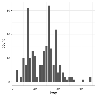
Tenga en cuenta que la geometría le dice a ggplot qué tipo de parcela usar, y la estadística (stat) le dice qué tipo de resumen presentar.
ggplot(mpg, aes(hwy)) +
  geom_line(stat = "density")