9.5: Puntuaciones Z

Última actualización
Guardar como PDF

Page ID: 150512

\( \newcommand{\vecs}[1]{\overset { \scriptstyle \rightharpoonup} {\mathbf{#1}} } \) \( \newcommand{\vecd}[1]{\overset{-\!-\!\rightharpoonup}{\vphantom{a}\smash {#1}}} \)\(\newcommand{\id}{\mathrm{id}}\) \( \newcommand{\Span}{\mathrm{span}}\) \( \newcommand{\kernel}{\mathrm{null}\,}\) \( \newcommand{\range}{\mathrm{range}\,}\) \( \newcommand{\RealPart}{\mathrm{Re}}\) \( \newcommand{\ImaginaryPart}{\mathrm{Im}}\) \( \newcommand{\Argument}{\mathrm{Arg}}\) \( \newcommand{\norm}[1]{\| #1 \|}\) \( \newcommand{\inner}[2]{\langle #1, #2 \rangle}\) \( \newcommand{\Span}{\mathrm{span}}\) \(\newcommand{\id}{\mathrm{id}}\) \( \newcommand{\Span}{\mathrm{span}}\) \( \newcommand{\kernel}{\mathrm{null}\,}\) \( \newcommand{\range}{\mathrm{range}\,}\) \( \newcommand{\RealPart}{\mathrm{Re}}\) \( \newcommand{\ImaginaryPart}{\mathrm{Im}}\) \( \newcommand{\Argument}{\mathrm{Arg}}\) \( \newcommand{\norm}[1]{\| #1 \|}\) \( \newcommand{\inner}[2]{\langle #1, #2 \rangle}\) \( \newcommand{\Span}{\mathrm{span}}\)\(\newcommand{\AA}{\unicode[.8,0]{x212B}}\)

Se obtiene una puntuación Z restando primero la media y luego dividiendo por la desviación estándar de una distribución. Hagamos esto para los datos height_sample.

mean_height <- mean(height_sample)
sd_height <- sd(height_sample)

z_height <- (height_sample - mean_height)/sd_height

Ahora vamos a trazar el histograma de las puntuaciones Z junto con el histograma para los valores originales. Usaremos la función plot_grid () de la biblioteca cowplot para trazar las dos figuras una junto a la otra. Primero necesitamos poner los valores en un marco de datos, ya que ggplot () requiere que los datos estén contenidos en un marco de datos.

height_df <- data.frame(orig_height=height_sample, 
                        z_height=z_height)

# create individual plots
plot_orig <- ggplot(height_df, aes(orig_height)) + 
  geom_histogram()
plot_z <- ggplot(height_df, aes(z_height)) + 
  geom_histogram()

# combine into a single figure
plot_grid(plot_orig, plot_z)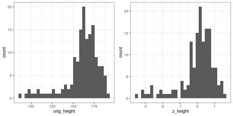

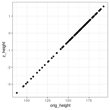
Notarás que las formas de los histogramas son similares pero no exactamente iguales. Esto ocurre porque el binning es ligeramente diferente entre los dos conjuntos de valores. Sin embargo, si los trazamos uno contra el otro en una gráfica de dispersión, veremos que existe una relación lineal directa entre los dos conjuntos de valores:

ggplot(height_df, aes(orig_height, z_height)) + 
  geom_point()