13.2: Teorema de Límite Central

Última actualización
Guardar como PDF

Page ID: 150711

\( \newcommand{\vecs}[1]{\overset { \scriptstyle \rightharpoonup} {\mathbf{#1}} } \) \( \newcommand{\vecd}[1]{\overset{-\!-\!\rightharpoonup}{\vphantom{a}\smash {#1}}} \)\(\newcommand{\id}{\mathrm{id}}\) \( \newcommand{\Span}{\mathrm{span}}\) \( \newcommand{\kernel}{\mathrm{null}\,}\) \( \newcommand{\range}{\mathrm{range}\,}\) \( \newcommand{\RealPart}{\mathrm{Re}}\) \( \newcommand{\ImaginaryPart}{\mathrm{Im}}\) \( \newcommand{\Argument}{\mathrm{Arg}}\) \( \newcommand{\norm}[1]{\| #1 \|}\) \( \newcommand{\inner}[2]{\langle #1, #2 \rangle}\) \( \newcommand{\Span}{\mathrm{span}}\) \(\newcommand{\id}{\mathrm{id}}\) \( \newcommand{\Span}{\mathrm{span}}\) \( \newcommand{\kernel}{\mathrm{null}\,}\) \( \newcommand{\range}{\mathrm{range}\,}\) \( \newcommand{\RealPart}{\mathrm{Re}}\) \( \newcommand{\ImaginaryPart}{\mathrm{Im}}\) \( \newcommand{\Argument}{\mathrm{Arg}}\) \( \newcommand{\norm}[1]{\| #1 \|}\) \( \newcommand{\inner}[2]{\langle #1, #2 \rangle}\) \( \newcommand{\Span}{\mathrm{span}}\)\(\newcommand{\AA}{\unicode[.8,0]{x212B}}\)

El teorema del límite central nos dice que la distribución muestral de la media se vuelve normal a medida que crece el tamaño de la muestra. Probemos esto muestreando una variable claramente no normal y veamos la normalidad de los resultados usando una gráfica Q-Q. Vimos en la Figura @ref {fig:Alcdist50} que la variable alcoholYear se distribuye de una manera muy no normal. Veamos primero la gráfica Q-Q para estos datos, para ver cómo se ve. Usaremos la función stat_qq () de ggplot2 para crear la gráfica para nosotros.

# prepare the dta
NHANES_cleanAlc <- NHANES %>%
  drop_na(AlcoholYear)

ggplot(NHANES_cleanAlc, aes(sample=AlcoholYear)) +
  stat_qq() + 
  # add the line for x=y
  stat_qq_line()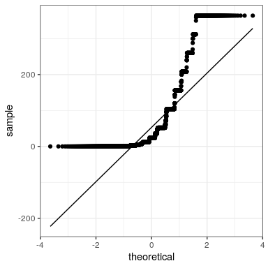

Podemos ver a partir de esta figura que la distribución es altamente no normal, ya que la gráfica Q-Q diverge sustancialmente de la línea unitaria.

Ahora vamos a muestrear y calcular repetidamente la media, y veamos la gráfica Q-Q resultante. Tomaremos muestras de varios tamaños para ver el efecto del tamaño de la muestra. Usaremos una función del paquete dplyr llamada do (), que puede ejecutar una gran cantidad de análisis a la vez.

set.seed(12345)

sampSizes <- c(16, 32, 64, 128) # size of sample
nsamps <- 1000 # number of samples we will take

# create the data frame that specifies the analyses
input_df <- tibble(sampSize=rep(sampSizes,nsamps),
                      id=seq(nsamps*length(sampSizes)))


# create a function that samples and returns the mean
# so that we can loop over it using replicate()
get_sample_mean <- function(sampSize){
  meanAlcYear <- 
    NHANES_cleanAlc %>%
    sample_n(sampSize) %>%
    summarize(meanAlcoholYear = mean(AlcoholYear)) %>%
    pull(meanAlcoholYear)
  return(tibble(meanAlcYear = meanAlcYear, sampSize=sampSize))
}

# loop through sample sizes
# we group by id so that each id will be run separately by do()
all_results = input_df %>% 
  group_by(id) %>%
  # "." refers to the data frame being passed in by do()
  do(get_sample_mean(.$sampSize))

Ahora vamos a crear parcelas Q-Q separadas para los diferentes tamaños de muestra.

# create empty list to store plots

qqplots = list()

for (N in sampSizes){
  sample_results <- 
    all_results %>%
    filter(sampSize==N)

  qqplots[[toString(N)]] <- ggplot(sample_results, 
                                aes(sample=meanAlcYear)) +
    stat_qq() + 
    # add the line for x=y
    stat_qq_line(fullrange = TRUE) + 
    ggtitle(sprintf('N = %d', N)) + 
   xlim(-4, 4) 

}

plot_grid(plotlist = qqplots)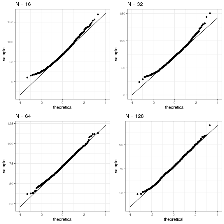

Esto demuestra que los resultados se distribuyen más normalmente (es decir, siguiendo la línea recta) a medida que las muestras se hacen más grandes.