5.10: Visibilidad de Flecos
- Page ID
- 130044
\( \newcommand{\vecs}[1]{\overset { \scriptstyle \rightharpoonup} {\mathbf{#1}} } \)
\( \newcommand{\vecd}[1]{\overset{-\!-\!\rightharpoonup}{\vphantom{a}\smash {#1}}} \)
\( \newcommand{\id}{\mathrm{id}}\) \( \newcommand{\Span}{\mathrm{span}}\)
( \newcommand{\kernel}{\mathrm{null}\,}\) \( \newcommand{\range}{\mathrm{range}\,}\)
\( \newcommand{\RealPart}{\mathrm{Re}}\) \( \newcommand{\ImaginaryPart}{\mathrm{Im}}\)
\( \newcommand{\Argument}{\mathrm{Arg}}\) \( \newcommand{\norm}[1]{\| #1 \|}\)
\( \newcommand{\inner}[2]{\langle #1, #2 \rangle}\)
\( \newcommand{\Span}{\mathrm{span}}\)
\( \newcommand{\id}{\mathrm{id}}\)
\( \newcommand{\Span}{\mathrm{span}}\)
\( \newcommand{\kernel}{\mathrm{null}\,}\)
\( \newcommand{\range}{\mathrm{range}\,}\)
\( \newcommand{\RealPart}{\mathrm{Re}}\)
\( \newcommand{\ImaginaryPart}{\mathrm{Im}}\)
\( \newcommand{\Argument}{\mathrm{Arg}}\)
\( \newcommand{\norm}[1]{\| #1 \|}\)
\( \newcommand{\inner}[2]{\langle #1, #2 \rangle}\)
\( \newcommand{\Span}{\mathrm{span}}\) \( \newcommand{\AA}{\unicode[.8,0]{x212B}}\)
\( \newcommand{\vectorA}[1]{\vec{#1}} % arrow\)
\( \newcommand{\vectorAt}[1]{\vec{\text{#1}}} % arrow\)
\( \newcommand{\vectorB}[1]{\overset { \scriptstyle \rightharpoonup} {\mathbf{#1}} } \)
\( \newcommand{\vectorC}[1]{\textbf{#1}} \)
\( \newcommand{\vectorD}[1]{\overrightarrow{#1}} \)
\( \newcommand{\vectorDt}[1]{\overrightarrow{\text{#1}}} \)
\( \newcommand{\vectE}[1]{\overset{-\!-\!\rightharpoonup}{\vphantom{a}\smash{\mathbf {#1}}}} \)
\( \newcommand{\vecs}[1]{\overset { \scriptstyle \rightharpoonup} {\mathbf{#1}} } \)
\( \newcommand{\vecd}[1]{\overset{-\!-\!\rightharpoonup}{\vphantom{a}\smash {#1}}} \)
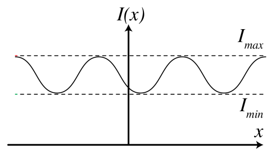
Hemos visto que cuando el término de interferencia\(\operatorname{Re}\left\langle U_{1}^{*} U_{2}\right\rangle\) desaparece, no se forman franjas, mientras que cuando este término es distinto de cero, hay franjas. La visibilidad de las franjas se expresa directamente en cantidades medibles (es decir, en intensidades en lugar de campos). Dado algún patrón de intensidad de interferencia\(I(x)\) como en la Figura\(\PageIndex{1}\), la visibilidad se define como\[\mathcal{V}=\frac{I_{\max }-I_{\min }}{I_{\max }+I_{\min }} . \quad \text { fringe visibility. } \nonumber \]
Por ejemplo, si tenemos dos fuentes puntuales monocromáticas perfectamente coherentes que emiten los campos\(U_{1}, U_{2}\) con intensidades\(I_{1}=\left|U_{1}\right|^{2}, I_{2}=\left|U_{2}\right|^{2}\), entonces el patrón de interferencia es con (5.6.13):\[I(\tau)=I_{1}+I_{2}+2 \sqrt{I_{1} I_{2}} \cos (\omega \tau+\varphi) . \nonumber \]
Entonces conseguimos\[I_{\max }=I_{1}+I_{2}+2 \sqrt{I_{1} I_{2}}, \quad I_{\min }=I_{1}+I_{2}-2 \sqrt{I_{1} I_{2}}, \nonumber \]\(\mathrm{SO}\)\[\mathcal{V}=\frac{2 \sqrt{I_{1} I_{2}}}{I_{1}+I_{2}} \nonumber \]
Por si acaso\(I_{1}=I_{2}\), nos encontramos\(\mathcal{V}=1\). En el caso contrario, donde\(U_{1}\) y\(U_{2}\) son completamente incoherentes, nos encontramos\[I(\tau)=I_{1}+I_{2}, \nonumber \] a partir del\[I_{\max }=I_{\min }=I_{1}+I_{2}, \nonumber \] cual sigue que da\(\mathcal{V}=0\).