13.10: Capítulo- 10

Problema (10.1).

(a) Usar el teorema de Stokes para mostrar que la ecuación de Maxwell\( \operatorname{curl} \mathbf{E}=-\frac{\partial \mathbf{B}}{\partial \mathrm{t}}\) puede escribirse en la forma

\[\oint_{C} \mathbf{E} \cdot d \mathbf{L}=-\frac{\partial}{\partial t} \quad \int_{\text {Surface S }} \mathbf{B} \cdot \mathbf{d} \mathbf{S} \quad \quad \quad \quad (1)\nonumber \]

donde la superficie S está delimitada por la curva cerrada c.

(b) Aplicar la ecuación anterior a un bucle que se extiende a ambos lados del límite entre dos materiales para demostrar que el componente tangencial de E debe ser continuo a través del límite.

Respuesta (10.1).

a)\(\text { curl } \mathbf{E}=-\frac{\partial \mathbf{B}}{\partial t}\)

Integrar sobre una superficie S delimitada por una curva c:

\(\int_{S} \operatorname{curl} \quad \mathbf{E} \cdot d \mathbf{S}=-\frac{\partial}{\partial t} \int_{S} \mathbf{B} \cdot d \mathbf{S}\)

Pero desde el teorema de Stokes

\(\int_{S} \operatorname{Curl } \mathbf{E} \cdot \mathrm{d} \mathbf{S}=\oint_{c}\mathbf{E} \cdot \mathrm{d} \mathbf{L}\), y el resultado sigue.

(b) Aplicar lo anterior a un bucle\(\delta\) L largo y de anchura insignificante,\(\delta\) d.

Entonces\(\oint_{c}\left.\left.\mathbf{E} \cdot \mathrm{d} \mathbf{L}=\mathrm{E}_{2}\right)_{\mathrm{tang}} \delta \mathrm{L}-\mathrm{E}_{1}\right)_{\mathrm{tang}} \delta \mathrm{L}\)

\(=-\frac{\partial}{\partial \mathrm{t}} \left(\mathrm{B}_{\mathrm{perp}}. \delta \mathrm{L} \delta \mathrm{d}\right) \Rightarrow 0\)

por lo tanto

\(\left.\left.\mathrm{E}_{2}\right)_{\mathrm{tangential}} =\mathrm{E}_{1}\right)_{\mathrm{tangential}}\)

Problema (10.2).

(a) Usar el teorema de Stokes para transformar la ecuación de Maxwell

\[\operatorname{curl} \mathbf{H}=\mathbf{J}_{\mathrm{f}}+\frac{\partial \mathbf{D}}{\partial \mathrm{t}}\nonumber\]

en

\[\underset{\mathrm{C}}{\oint} \mathbf{H} \cdot \mathrm{d} \mathbf{L}=\int_{\mathrm{S}}\left(\mathbf{J}_{\mathrm{f}}+\frac{\partial \mathbf{D}}{\partial \mathrm{t}}\right) \cdot \mathrm{d} \mathbf{S}, \nonumber\]

donde la superficie S está delimitada por la curva cerrada, c.

(b) Utilizar la ecuación anterior para mostrar que en la superficie de discontinuidad entre dos materiales el componente tangencial de H debe ser continuo.

Respuesta (10.2).

a)\(\operatorname{Curl} \mathbf{H} \quad=\quad\left(\mathbf{J}_{\mathrm{f}}+\frac{\partial \mathbf{D}}{\partial \mathrm{t}}\right)\)

\(\therefore \quad \int_{S} \operatorname{Curl} \mathbf{H} \cdot \mathrm{d} \mathbf{S}=\int_{S} \mathbf{J}_{f} \cdot \mathrm{d} \mathbf{S}+\frac{\partial}{\partial \mathrm{t}} \int_{\mathrm{S}} \mathbf{D} \cdot \mathrm{d} \mathbf{S}.\)

Pero por el teorema de Stokes:

\[\int_{S} \operatorname{Curl} \mathbf{H} \cdot \mathrm{d} \mathbf{S}=\underset{\mathrm{c}}{\oint} \mathbf{H} \cdot \mathrm{d} \mathbf{L} \nonumber\]

de la que se desprende el resultado.

(b) Aplicar el teorema anterior a un bucle que se extiende a ambos lados del límite. El bucle es\(\delta\) L largo y\(\delta\) d ancho.

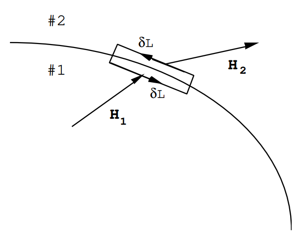
\(\left.\left.\oint_{c}{\delta \mathbf{H}} \cdot \mathrm{d} \mathbf{L}=\mathrm{H}_{2}\right)_{\mathrm{tang}} \delta \mathrm{L}-\mathrm{H}_{1}\right)_{\mathrm{tang}} \delta \mathrm{L}+\text { terms } 2 \mathrm{nd} \text { order in } \delta \mathrm{d}\)

\(\int_{S}\left(J_{f}+\frac{\partial D}{\partial t}\right) \cdot d s=\left(J_{f}+\frac{\partial D}{\partial t}\right)_{\text {normal }} \delta L \delta d \Rightarrow 0 \text { as } \delta d \rightarrow 0\)

\(\begin{equation}\left.\left.\therefore \quad \mathrm{H}_{2}\right)_{\mathrm{tang}}=\mathrm{H}_{1}\right)_{\mathrm{tang}}\end{equation}\)

Problema (10.3).

1. De div B = 0 muestran que el componente normal de B es continuo a través del límite entre dos materiales diferentes.
2. De div D = ρ _f muestran que habrá una densidad de carga superficial en la superficie de discontinuidad entre dos materiales. Mostrar que la magnitud de esta densidad de carga superficial viene dada por

\[\begin{equation}\left.\left.\rho_{\mathrm{f}}=\mathrm{D}_{2}\right)_{\text {normal }}-\mathrm{D}_{1}\right)_{\text {normal }}\end{equation}\nonumber\]

donde\(\left.\mathrm{D}_{2}\right)_{\text {normal }}\) y\(\left.\mathrm{D}_{1}\right)_{\text {normal }}\) son los componentes normales del vector D.

Respuesta (10.3).

(a)\(\operatorname{div} \mathbf{B}=0\)

\(\therefore \int_{V} \mathrm {div} \textbf{B } d \tau=0\)

Pero por el teorema de Gauss\(\int_{V} \mathrm{div} \textbf{B } d \tau=\int_{S} \mathbf{B} \cdot d \mathbf{S}\)

donde S es la superficie que delimita el volumen cerrado V.

Por lo tanto\(\int_{S} \mathbf{B} \cdot d \mathbf{S}=0\)

Aplicar esto a una caja de pastillas de área\(\delta\) A y espesor\(\delta\) L que se extiende a ambos lados del límite entre el material (1) y el material (2)

\(\left.\left.\int_{\operatorname{Pill Box}} \underset{\mathrm{box}}{\mathbf{B} \cdot \mathrm{d} \mathbf{S}}=\left[\mathrm{B}_{2}\right)_{\text {normal }}-\mathrm{B}_{1}\right)_{\text {normal }}\right] \delta A + \text{ terms of 2nd order in } \delta L\)

(Como se muestra,\(\mathbf{B}_{2} \cdot \hat{\mathbf{u}}_{2}\) hace una contribución positiva y\(\mathbf{B}_{1} \cdot \hat{\mathbf{u}}_{1}\) hace una contribución negativa).

Por lo tanto,\(\left.\left.\left[\mathrm{B}_{2}\right)_{\text {normal }}-\mathrm{B}_{1}\right)_{\text {normal }}\right] \delta \mathrm{A}=0\) para arbitrarios\(\delta\) A y

\[\therefore \left.\left.\mathrm{B}_{2}\right)_{\text {normal }}=\mathrm{B}_{1}\right)_{\text {normal }}\nonumber\]

(b) div D = ρ _f

* para cualquier volumen cerrado V delimitado por una superficie S

\(\int_{V} \mathrm{div} \textbf{D } d \tau=\int_{V} \rho_{f} d \tau\)

Pero según el teorema de Gauss:

\(\int_{V}(d i v \mathbf{D}) d \tau=\int_{S} \mathbf{D \cdot d s}\)

Aplica esto a una caja de paletas que se extiende sobre el material (1) y el material (2):

Entonces\(\left.\left.\int_{\mathrm{S}} \mathrm{D} \cdot \mathrm{d} \mathrm{s}=\left[\mathrm{D}_{2}\right)_{\text {normal }} \delta \mathrm{A}-\mathrm{D}_{1}\right)_{\text {normal }} \delta \mathrm{A}\right]\)

+ correcciones de orden superior del orden\(\delta\) L\(\delta\) A.

\(\left.\left.\therefore\left[\mathrm{D}_{2}\right)_{\text {normal }}-\mathrm{D}_{1}\right)_{\text {normal }}\right]\delta \mathrm{A}=\rho_{\mathrm{f}} \delta \mathrm{A} \delta \mathrm{L}\)

Entonces\(\left.\left.\left[\mathrm{D}_{2}\right)_{\text {normal }}-\mathrm{D}_{1}\right)_{\text {normal }}\right]=\rho_{\mathrm{f}} \delta \mathrm{L}=\rho_{\mathrm{s}}\),

donde (ρ _{f\(\delta\) L}) no depende de la longitud\(\delta\) _L y por lo tanto representa una carga superficial ρ _s. Una discontinuidad en el componente normal de D significa que existe una densidad de carga superficial.

Problema (10.4).

Una ola plana cae con incidencia normal en la superficie plana de un cuerpo de agua grande y profundo. Las partes real e imaginaria del índice de refracción para el agua son n = 4/3 y\(\kappa\) = 10 ^-8 correspondientes a una dependencia del tiempo ~ e ^-iωt. La amplitud del campo eléctrico en la onda incidente es de 1 V/m. Deje que el eje z se dirija al agua y deje que los ejes x, y se encuentren en la superficie del agua. Dejar polarizar el campo eléctrico a lo largo de x. El índice de refracción del aire es n = 1,\(\kappa\) = 0.

1. Escribir una ecuación para la variación de espacio y tiempo del campo eléctrico en la onda incidente.
2. Escribe una ecuación para las variaciones de espacio y tiempo de B, H en la onda incidente. ¿Cuál es la amplitud, H _o, del campo H?
3. Escribir expresiones para la variación de espacio y tiempo de la onda reflejada. Deje que la amplitud del campo eléctrico reflejado sea E _R. Escribe la amplitud del campo magnético reflejado en términos de E _R.
4. Escribir expresiones para las variaciones de espacio y tiempo de las ondas de campo eléctrico y magnético (campo H) transmitidas al agua. Deje que la amplitud del campo eléctrico en la superficie del agua, a z = 0, sea E _T. Escribe la amplitud del campo magnético en términos de E _T.
5. Indicar las condiciones límite que E, H debe satisfacer en la superficie del agua.
6. Aplicar las condiciones límite de la parte (e) para obtener la amplitud del campo eléctrico reflejado, E _R, y la amplitud del campo eléctrico de onda transmitida, E _T.
7. ¿Cuál es la intensidad de la ola incidente? es decir, ¿a qué velocidad, en vatios/m ², se transporta la energía a la superficie del agua?
8. ¿A qué ritmo es la energía absorbida por el agua?
9. ¿Cuál será la amplitud del campo eléctrico a una profundidad de 2 m si la longitud de onda de la luz es de 1/2 micrón?

Respuesta (10.4).

(a)

b)\(B_{y}=\frac{E_{x}}{c}=\frac{1}{c} e^{i(k z-\omega t)}\)

\(\mathrm{H}_{\mathrm{y}}=\frac{\mathrm{B}_{\mathrm{Y}}}{\mu_{\mathrm{O}}}=\frac{1}{\mathrm{c} \mu_{\mathrm{O}}} e^{\mathrm{i}(\mathrm{kz}-\omega \mathrm{t})}=\frac{1}{120 \pi} \mathrm{e}^{\mathrm{i}(\mathrm{kz}-\omega \mathrm{t})} \quad \mathrm{Amps} / \mathrm{m}\).

\(\text { Amplitude }=\frac{1}{120 \pi}=\frac{1}{377} \text { Amps } / \mathrm{m}\).

c) Dejar que el campo eléctrico reflejado sea

\(E_{x}=E_{R} e^{-i(k z+\omega t)}\)

(nota cambio en signo de k).

Entonces\(\mathrm{H}_{\mathrm{y}}=-\frac{\mathrm{E}_{\mathrm{R}}}{120 \pi} \mathrm{e}^{-\mathrm{i}(\mathrm{kz}+\omega \mathrm{t})}\)

d) En el agua el vector de propagación viene dado por\(\mathrm{k}=\frac{\omega}{\mathrm{c}}(\mathrm{n}+\mathrm{i} \kappa)\)

\(\therefore \mathrm{E}_{\mathrm{X}}=\mathrm{E}_{\mathrm{T}} e^{-\kappa \frac{\omega}{c} z}e^{i\left(\frac{n \omega_{z}}{c}-\omega t\right)}\)

Ahora\(\operatorname{curl} \mathbf{E}=-\frac{\partial \mathbf{B}}{\partial \mathrm{t}}=\mathrm{i} \omega \mathbf{B}=\mathrm{i} \omega \mu_{\mathrm{o}} \mathbf{H}\)

\(\mathrm{i} \omega \mu_{\mathrm{O}} \mathbf{H}=\left|\begin{array}{ccc}\hat{\mathbf{u}}_{\mathrm{x}} & \hat{\mathbf{u}}_{\mathrm{y}} & \hat{\mathbf{u}}_{\mathrm{z}} \\0 & 0 & \frac{\partial}{\partial \mathrm{z}} \\ \mathrm{E}_{\mathrm{x}} & 0 & 0 \end{array}\right|=\left|\begin{array}{c} 0 \\ \frac{\partial \mathrm{E}_{\mathrm{x}}}{\partial \mathrm{z}} \\ 0 \end{array}\right|\)

\(\therefore \mathrm{H}_{\mathrm{Y}}=\frac{1}{\mathrm{i} \omega \mu_{\mathrm{o}}} \frac{\partial \mathrm{E}_{\mathrm{x}}}{\partial \mathrm{z}}=\frac{\mathrm{i}\left(\frac{\omega}{\mathrm{c}}\right)(\mathrm{n}+\mathrm{i} \kappa) \mathrm{E}_{\mathrm{X}}}{\mathrm{i} \omega \mathrm{u}_{\mathrm{O}}}=\frac{(\mathrm{n}+\mathrm{i} \kappa)}{\mu_{\mathrm{O}} \mathrm{c}} \mathrm{E}_{\mathrm{X}}\)

y

\(\mathrm{H}_{\mathrm{y}}=\left(\frac{\mathrm{n}+\mathrm{i} \kappa}{\mu_{\mathrm{O}} \mathrm{c}}\right) \mathrm{E}_{\mathrm{T}} e^{-\kappa \frac{\omega_{z}}{\mathrm{c}}} e^{\mathrm{i}\left(\mathrm{n} \frac{\omega_{z}}{\mathrm{c}}-\omega t\right)}.\)

e) En la interfaz, las condiciones límite requeridas son

(1) Los componentes tangenciales de E deben ser continuos.

(2) Los componentes tangenciales de H deben ser continuos.

(f) A z = 0

Ola Incidente\(E_{x}=(1) e^{-i \omega t}\)

\(\mathrm{H}_{\mathrm{y}}=\frac{1}{\mathrm{c} \mu_{0}} \mathrm{e}^{-\mathrm{i} \omega \mathrm{t}}\)

Onda Reflejada\(E_{x}=E_{R} e^{-i \omega t}\)

\(\mathrm{H}_{\mathrm{Y}}=-\frac{\mathrm{E}_{\mathrm{R}}}{\mathrm{c} \mu_{\mathrm{O}}} e^{-\mathrm{i} \omega \mathrm{t}}\)

Onda Transmitida\(E_{x}=E_{T} e^{-i \omega t}\)

\(\mathrm{H}_{\mathrm{Y}}=\frac{(\mathrm{n}+\mathrm{i} \kappa)}{\mathrm{c} \mu_{\mathrm{O}}} \mathrm{E}_{\mathrm{T}} e^{-\mathrm{i} \omega \mathrm{t}}\)

Continuidad de E _x:\(1+\mathrm{E}_{\mathrm{R}}=\mathrm{E}_{\mathrm{T}} \quad \quad \quad \quad (1) \)

Continuidad de H _y:\(\frac{1}{\mathrm{c} \mu_{0}}-\frac{\mathrm{E}_{\mathrm{R}}}{\mathrm{c} \mu_{0}}=\frac{(\mathrm{n}+\mathrm{i} \kappa)}{\mathrm{c} \mu_{0}} \mathrm{E}_{\mathrm{T}}\)

o\(1-\mathrm{E}_{\mathrm{R}}=(\mathrm{n}+\mathrm{i} \kappa) \mathrm{E}_{\mathrm{T}} \quad \quad \quad \quad (2) \)

Resuelve eqns. (1) y (2) para obtener:

\(E_{T}=\frac{2}{(1+n)+i \kappa}=\frac{2[(n+1)-i \kappa]}{(n+1)^{2}+\kappa^{2}}\)

Pero\(\kappa \simeq 0\) así\(E_{T}=\frac{14 / 3}{(7 / 3)^{2}}=\frac{6}{7}= \underline {0.86 \ Volts / m.}\)

También\(E_{T} \simeq\left(\frac{2}{n+1}\right)\)

y\(\mathrm{E}_{\mathrm{R}}=\mathrm{E}_{\mathrm{T}}-1=\underline{-0.143 \ Volts / m.}\)

(NOTA EL CAMBIO DE FASE EN EL CAMPO ELÉCTRICO!!)

g) La tasa de transporte de energía a la superficie del agua es

\(\mathrm{S}_{\mathrm{z}}=\mathrm{E}_{\mathrm{x}} \mathrm{H}_{\mathrm{y}}\)

\(\begin{aligned} \left\langle S_{z}\right\rangle &=\left(\frac{1}{2}\right)(1)\left(\frac{1}{c \mu_{0}}\right)=\frac{1}{754} \text { Watts } / \mathrm{m}^{2} \\ &=\underline{1.33 \ {mW} / {m}^{2}.} \end{aligned}\)

h) La tasa de energía reflejada desde la superficie es

\(<S_{z}>_{R}=\frac{1}{2}\left(E_{R}\right) \frac{\left(E_{R}\right)}{c \mu_{0}}=\frac{(0.143)^{2}}{754}=\underline{0.027 \ \mathrm{mW} / \mathrm{m}^{2}}= \underline{27 \ \mathrm{\mu W} / \mathrm{m}^{2}.}\)

∙Energía absorbida en H ₂ O = 1.30 mW/m ².

(i) A z = 2m

\(\left|\mathrm{E}_{\mathrm{X}}\right|=\mathrm{E}_{\mathrm{T}} \mathrm{e}^{-\kappa 4 \pi / \lambda}=\mathrm{E}_{\mathrm{T}} \mathrm{e}^{-0.251}=0.78 \ \mathrm{E}_{\mathrm{T}}\)

⟩ @ 2m la intensidad del campo eléctrico = 0.67 V/m.

Problema (10.5).

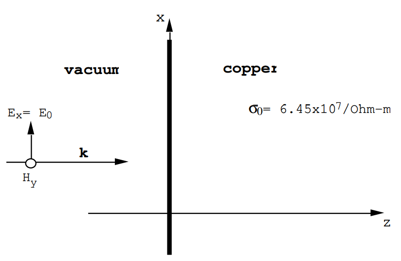
Una onda que tiene una amplitud de campo eléctrico E _o = 1 V/m cae a incidencia normal sobre una superficie plana de cobre como se muestra en el boceto anterior. Su frecuencia es de 10 ⁶ Hz.

1. Escribir expresiones para los campos eléctricos y magnéticos en la onda incidente. ¿Qué tan grande es H _y?
2. Calcular la magnitud del vector de onda de vacío.
3. Calcular el vector de onda en el metal (k _m) en las expresiones:\[E_{x}=E_{T} e^{i\left(\mathrm{k}_{m} z-\omega t\right)}\nonumber\]\[\mathrm{H}_{\mathrm{Y}}=\mathrm{H}_{\mathrm{T}} \mathrm{e}^{\mathrm{i}\left(\mathrm{k}_{\mathrm{m}} \mathrm{z}-\omega \mathrm{t}\right)}\nonumber\]
4. Calcular la amplitud del campo eléctrico en la superficie del metal es decir E _T.
5. Calcular la amplitud del campo magnético en la superficie del metal es decir H _T.
6. Calcular el tiempo promedio del vector de Poynting para la onda incidente, es decir <S _o >
7. Calcular el tiempo promedio del vector de Poynting para el flujo de energía en el metal, es decir <S _m >
8. De (f) y (g) calcular el coeficiente de absorción\(\alpha\) = <S _m >/<S _o >.
9. Calcular la tasa promedio de disipación de energía como calor Joule en el metal. Mostrar que la integral de esta cantidad de z = o a ∞ es justo igual a <S _m > de (g) anterior.

Respuesta (10.5).

(a)\(\mathrm{k}=\frac{\omega}{c}=\frac{2 \pi \times 10^{6}}{3 \times 10^{8}}=\mathbf{2.094 \times 10^{-2}\ \mathbf{m}^{-1}}\)

\(E_{x}=E_{0} e^{i(k z-\omega t)}=e^{i(k z-\omega t)}\)ya que E _o = 1 V/m.

\(\mathrm{H}_{\mathrm{Y}}=\frac{\mathrm{E}_{0}}{\mathrm{Z}_{\mathrm{0}}} e^{\mathrm{i}(\mathrm{k} \mathrm{z}-\omega \mathrm{t})}=\mathbf{\left(2.653 \times 10^{-3}\right)} \ \mathrm{e}^{\mathrm{i}(\mathrm{kz}-\omega \mathrm{t})}\)

desde Z _o = 377 Ohmios.

(b) Ver arriba. k = 2.094 x 10 ^-2 /metro.

c) En el metal:

\ (\ nombreoperador {rizo}\ mathbf {E} =\ izquierda|\ begin {array} {ccc}
\ hat {\ mathbf {u}} _ {\ mathbf {x}} &\ hat {\ mathbf {u}} _ {y} &\ hat {\ mathbf {u}} _ {z}\
0 &\ frac {\ parcial} {\ parcial}}\\
E_ {x} & 0 & 0
\ end {array}\ derecha|=\ izquierda|\ begin {array} {c }
0\\
\ frac {\ parcial E_ {x}} {\ z parcial}\\
0
\ final {array}\ derecha|=i\ omega\ mu_ {0}\ mathbf {H},\)

\(\operatorname{curl} \mathbf{H}=\left|\begin{array}{ccc}\hat{\mathbf{u}}_{\mathbf{x}} & \hat{\mathbf{u}}_{y} & \hat{\mathbf{u}}_{z} \\ 0 & 0 & \frac{\partial}{\partial z} \\ 0 & \mathrm{H}_{\mathrm{y}} & 0 \end{array}\right|=\left|\begin{array}{c} -\frac{\partial \mathrm{H}_{\mathrm{y}}}{\partial \mathrm{z}} \\ 0 \\ 0 \end{array}\right|=\sigma \mathbf{E}.\)

\(\therefore \frac{\partial E_{x}}{\partial z}=i \omega \mu_{0} H_{y}=i k_{m} E_{x}\)

o\(\mathbf{H_{y}=\left(\frac{\mathbf{k}_{m}}{\omega \mu_{0}}\right) \mathbf{E}_{\mathbf{x}}}\)

y\(\frac{\partial \mathrm{H}_{\mathrm{Y}}}{\partial \mathrm{z}}=-\sigma \mathrm{E}_{\mathrm{X}}\)

\(\mathrm{i} \mathrm{k}_{\mathrm{m}} \mathrm{H}_{\mathrm{y}}=-\sigma \mathrm{E}_{\mathrm{x}}\)

o\(\mathbf{H_{y}=\left(\frac{i \sigma}{k_{m}}\right)E_{x}}\).

Así\(\frac{\mathrm{i} \sigma}{\mathrm{k}_{\mathrm{m}}}=\frac{\mathrm{k}_{\mathrm{m}}}{\omega \mu_{\mathrm{o}}}\) o\(k_{m}^{2}=i \omega \mu_{0} \sigma\)

\(k_{m}^{2}=i\left(2 \pi \times 10^{6}\right)\left(4 \pi \times 10^{-7}\right)\left(6.45 \times 10^{7}\right)\)

= i (5.093 x 10 ⁸)

\({k}_{m}=\left(\frac{1+{i}}{\sqrt{2}}\right)\left(2.257 \times 10^{4}\right)=\mathbf{\left(1.596 \times 10^{4}\right)(1+{i})}.\)

N.B. km es muy grande c.f. k = ω/c. aprox. 10 ⁶ más grande!!

A z = 0: a) Continuidad de E _x:\(\mathrm{E}_{\mathrm{O}}+\mathrm{E}_{\mathrm{R}}=\mathrm{E}_{\mathrm{T}}\)

b) Continuidad de H _y:\(\frac{E_{0}}{Z_{0}}-\frac{E_{R}}{Z_{0}}=H_{T}\)

o\(\mathrm{E}_{\mathrm{O}}-\mathrm{E}_{\mathrm{R}}=\mathrm{Z}_{\mathrm{O}} \mathrm{H}_{\mathrm{T}}\)

\(\therefore 2 \mathrm{E}_{\mathrm{O}}=\left(\mathrm{E}_{\mathrm{T}}+\mathrm{Z}_{\mathrm{O}} \mathrm{H}_{\mathrm{T}}\right)=\left[1+\frac{\mathrm{i} \sigma \mathrm{z}_{\mathrm{O}}}{\mathrm{k}_{\mathrm{m}}}\right] \mathrm{E}_{\mathrm{T}}\)

\(2 \mathrm{E}_{\mathrm{R}}=\left(\mathrm{E}_{\mathrm{T}}-\mathrm{Z}_{\mathrm{O}} \mathrm{H}_{\mathrm{T}}\right)=\left[1-\frac{\mathrm{i} \sigma \mathrm{Z}_{\mathrm{O}}}{\mathrm{k}_{\mathrm{m}}}\right] \mathrm{E}_{\mathrm{T}}\)

Pero\(\mathrm{H}_{\mathrm{T}}=\left(\frac{\mathrm{i} \sigma}{\mathrm{k}_{\mathrm{m}}}\right) \mathrm{E}_{\mathrm{T}}\)

\(\therefore \frac{E_{R}}{E_{0}}=\frac{1-\frac{i \sigma Z_{0}}{k_{m}}}{1+\frac{i \sigma Z_{0}}{k_{m}}}\)\(\frac{E_{T}}{E_{0}}=\frac{2}{1+\frac{i \sigma Z_{0}}{k_{m}}}\).

\(\frac{1}{k_{m}}=\left(\frac{10}{1.596}\right) \times 10^{-5}\left(\frac{1}{1+i}\right)=\left(\frac{5 \times 10^{-5}}{1.596}\right)(1-i)\)

\(=3.133(1-i) \times 10^{-5}\)

\(\therefore\left(\frac{\mathrm{i}}{\mathrm{k}_{\mathrm{m}}}\right)=\mathbf{\left(3.133 \times 10^{-5}\right) (1+{i})}\).

Entonces\(\frac{i \sigma Z_{0}}{k_{m}}=(3.133)\left(10^{-5}\right)\left(6.45 \times 10^{7}\right)(377)(1+i)\)

\(=\mathbf{\left(7.618 \times 10^{5}\right)(1+i)}\).

Esto es mucho mayor que 1.

\(\therefore \frac{E_{T}}{E_{0}} \cong \frac{2}{\frac{i \sigma Z_{0}}{k_{m}}}=\frac{-i 2 k_{m}}{\sigma Z_{0}}=\mathbf{1.313 \times 10^{-6}(1-i).}\)

\(\frac{E_{R}}{E_{0}}=\frac{-\left[1+\frac{i k_{m}}{\sigma Z_{0}}\right]}{\left[1-\frac{i k_{m}}{\sigma Z_{0}}\right]} \simeq-\left[1+\frac{2 i k_{m}}{\sigma Z_{0}}\right] \cong-1\)

a aproximadamente 1 parte en 10 ⁶!

e) De la parte (c)\(\mathrm{H}_{\mathrm{Y}}=\left(\frac{\mathrm{i} \sigma}{\mathrm{k}_{\mathrm{m}}}\right) \mathrm{E}_{\mathrm{X}}\)\(\left.\therefore \mathrm{H}_{\mathrm{T}}=\frac{\mathrm{i} \sigma}{\mathrm{k}_{\mathrm{m}}}\right) \quad \mathrm{E}_{\mathrm{T}}\)

y\(\mathrm{H}_{\mathrm{T}} \cong\left(\frac{\mathrm{i} \sigma}{\mathrm{k}_{\mathrm{m}}}\left(-\mathrm{i} \frac{2}{\sigma} \frac{\mathrm{k}_{\mathrm{m}}}{\mathrm{Z}_{\mathrm{0}}}\right)= \frac{2}{\mathrm{z}_{\mathrm{0}}}\right.\)

N.B. a primer orden en\(\left(\frac{2}{\sigma} \frac{\mathrm{k}_{\mathrm{m}}}{\mathrm{Z}_{\mathrm{0}}}\right)\) la amplitud del campo magnético en el metal es INDEPENDIENTE de\(\sigma\), ω!!

El factor 2 proviene de la suma H _T = H _o + H _R, donde\(\mathrm{H}_{\mathrm{0}}=\frac{\mathrm{E}_{\mathrm{0}}}{\mathrm{Z}_{\mathrm{0}}}\) &\(\mathrm{H}_{\mathrm{R}}=\frac{\left|\mathrm{E}_{\mathrm{R}}\right|}{\mathrm{Z}_{\mathrm{0}}}\)

Pero E _o = 1 V/m & E _R = -1 v/m (a 1 parte en 10 ⁶)

\(\therefore \mathrm{H}_{\mathrm{T}}=\frac{2}{\mathrm{Z}_{\mathrm{0}}}=\mathbf{5.305 \times 10^{-3} \ {Amps} / {m}.}\)

f) Por la ola incidente\(\left\langle\mathrm{S}_{\mathrm{0}}\right\rangle=\frac{1}{2} \ \operatorname{Real} \ \left\{\mathrm{E}_{\mathrm{X}} \mathrm{H}_{\mathrm{Y}}^{*}\right\}\)

\(=\frac{\mathrm{E}_{0}^{2}}{2 \mathrm{z}_{0}}=\frac{1}{2 \mathrm{z}_{0}}=\mathbf{1.326 \times 10^{-3} \ {watts} /{m}^{2}.}\)

(g) En la superficie metálica (z = 0)

\[\begin{aligned} \left\langle S_{m}\right\rangle &=\frac{1}{2} \text { Real }\left\{E_{T} H_{T} ^*\right\} \\ &=\frac{1}{2} \operatorname{Real} \left\{\left(1.313 \times 10^{-6}\right)(1-i) \frac{(2)}{Z_{0}}\right\} \\ &=\left(\frac{1.313}{Z_{0}} \times 10^{-6}\right)= \mathbf{3.48 \times 10^{-9} \ Watts / m^{2}.} \end{aligned}\nonumber\]

h)\(\alpha=\left\langle S_{m}\right\rangle /\left\langle S_{0}\right\rangle=\frac{3.48}{1.326} \times 10^{-6}=\mathbf{2.627 \times 10^{-6}.}\)

(i) En el metal la densidad de corriente viene dada por

\(\mathrm{J}_{\mathrm{x}}=\sigma \mathrm{E}_{\mathrm{x}}=\sigma \mathrm{E}_{\mathrm{T}} e^{\mathrm{i}\left(\mathrm{k}_{\mathrm{m}} \mathrm{z}-\omega \mathrm{t}\right)}\)

El calor/volumen de Joule (promedio de tiempo) es

\[\begin{aligned}\frac{d Q}{d t}&=\frac{1}{2} \operatorname{Real}\left\{J_{x} E_{x}^{*}\right\} \\\quad &=\frac{1}{2} \operatorname{Real}\left\{\sigma E_{T} e^{i\left(k_{m} z-\omega t\right)} \cdot E_{T}^{*} e^{-i\left(k_{m}^{*} z-\omega t\right)}\right\} \\ \quad &=\frac{1}{2} \operatorname{Real}\left\{\sigma\left|E_{T}\right|^{2} e^{i\left(k_{m}-k_{m}^{*}\right) z}\right\}\end{aligned}\nonumber\]

Pero\(\mathrm{k}_{\mathrm{m}}=\gamma(1+\mathrm{i})\) y\(\mathrm{k}_{\mathrm{m}}^{*}=\gamma(1-\mathrm{i}) \quad \quad \quad \therefore \mathrm{k}_{\mathrm{m}}-\mathrm{k}_{\mathrm{m}}^{*}=2 \mathrm{i} \gamma\)

y\(\gamma\) = 1.596 x 10 ⁴ de la parte (c)

&\(\mathrm{i}\left(\mathrm{k}_{\mathrm{m}}-\mathrm{k}_{\mathrm{m}}^{*}\right)=-2 \gamma\)

\(\therefore \frac{d Q}{d t}=\mathbf{\frac{\sigma}{2}\left|E_{T}\right|^{2} e^{-2 \gamma z}.}\)

Tasa total de producción de calor\(=\frac{\sigma\left|E_{T}\right|^{2}}{2} \int_{0}^{\infty} e^{-2 \gamma z} d z=\frac{\sigma\left|E_{T}\right|^{2}}{4 \gamma}.\)

\(\left.\therefore Q_{\text {Total }}=\frac{\left(6.45 \times 10^{7}\right)}{(4)\left(1.596 \times 10^{4}\right)}(1.313)^{2} \times 10^{-12}\right.)(2)=\mathbf{3.48 \times 10^{-9}\ Watts/m^{2}.}\)

\(=<\mathrm{S}_{\mathrm{m}}>(\text { from }(\mathrm{g}))\).

Problema (10.6).

La luz que tiene una longitud de onda de 5145 Å (0.5145 µm) cae sobre una superficie plana de cobre con incidencia normal. La intensidad de la luz es de 10 ⁵ vatios/m ² (es decir, 100 mW en un rayo láser de 1x1 mm en sección transversal). El complejo índice de refracción para el cobre a 5145 Å es\(\sqrt{\varepsilon_{r}}=(1.19+2.60 i)\) para una dependencia del tiempo de e ^-iωt.

a) Calcular las amplitudes de los campos eléctrico y magnético en la onda incidente.

(b) Calcular las amplitudes de los campos eléctrico y magnético en la onda reflejada.

(c) Calcular la intensidad de la onda reflejada; es decir, calcular el valor promediado en el tiempo del vector Poynting.

d) Calcular el vector de onda de la luz en el cobre. ¿Cuál es la velocidad de fase asociada a la onda en el cobre?

(e) Calcular las amplitudes de los campos eléctrico y magnético en el cobre pero cerca de la superficie en z=0.

(f) Calcular el valor promedio de tiempo del vector Poynting dentro del cobre pero cerca de la superficie en z=0.

g) ¿Hasta qué punto penetra la luz en el cobre antes de que su intensidad haya disminuido al 1% de su intensidad en la superficie?

(h) Calcular la densidad de energía promediada en el tiempo<W>,, almacenada en los campos eléctrico y magnético en el cobre pero en la superficie z=0. Demuestre que\(\left\langle\mathrm{S}_{\mathrm{z}}\right\rangle=\frac{\mathrm{c}}{\mathrm{n}}<\mathrm{W}>\) Watts/m ².

Respuesta (10.6).

a) Ola incidente:

\[E_{x}=E_{0} e^{i(k z-\omega t)}\nonumber\]

\[\mathrm{H}_{\mathrm{y}}=\frac{\mathrm{E}_{0}}{\mathrm{Z}_{0}} e^{\mathrm{i}(\mathrm{kz}-\omega \mathrm{t})}, \nonumber\]

donde k= ω/c y Z ₀ = µ ₀ c = 377 Ohmios.

\(<\mathrm{S}_{\mathrm{z}}>=\frac{1}{2} \operatorname{Real}\left(\mathrm{E}_{\mathrm{x}} \mathrm{H}_{\mathrm{y}}^{*}\right)=\frac{\mathrm{E}_{0}^{2}}{2 \mathrm{Z}_{0}}=\mathrm{I}_{0}=10^{5} \text { Watts } / \mathrm{m}^{2}.\)

Por lo tanto\(\mathrm{E}_{0}^{2}=75.4 \times 10^{6}\),, y E ₀ = 8.683x10 ³ Voltios/m, y H _y = 23.03 Amps/m.

b) A partir del problema del valor límite

\[\frac{E_{R}}{E_{0}}=\frac{1-\sqrt{\varepsilon}}{1+\sqrt{\varepsilon}}=\frac{(1-n)-i \kappa}{1+n+i \kappa}=r.\nonumber\]

Para este problema n=1.19 y\(\kappa\) =2.60;

r = -0.621- 0.45i, y por lo tanto r= - Re ^i\(\phi\) donde R=0.767, y Tan\(\phi\) = 0.725 de manera que\(\phi\) = 35.93° = 0.627 radianes. El signo menos significa que la dirección de la amplitud de onda reflejada se invierte en relación con la amplitud en la onda incidente.

\[\left|E_{R}\right|=R\left|E_{0}\right|=6.66 \times 10^{3} \ \mathrm{V} / \mathrm{m},\nonumber\]

y

\[\left|\mathrm{H}_{\mathrm{R}}\right|=\mathrm{R}\left|\mathrm{H}_{\mathrm{y}}\right|=17.66 \ \mathrm{Amps} / \mathrm{m}.\nonumber\]

c) La intensidad de la onda reflejada viene dada por

\[\mathrm{I}_{\mathrm{R}}=\mathrm{R}^{2} \mathrm{I}_{0}=0.588 \times 10^{5} \text { Watts } / \mathrm{m}^{2}. \nonumber\]

d) En el cobre\(\mathrm{k}_{\mathrm{m}}^{2}=\varepsilon_{\mathrm{r}}\left(\frac{\omega}{\mathrm{c}}\right)^{2}\)

\[\mathrm{k}=\frac{\omega}{\mathrm{c}}=\frac{2 \pi}{\lambda}=1.221 \times 10^{7} \mathrm{m}^{-1}. \nonumber\]

\[\mathrm{k}_{\mathrm{m}}=(\mathrm{n}+\mathrm{i} \mathrm{k}) \frac{\omega}{\mathrm{c}}=(1.453+\mathrm{i} 3.175) \times 10^{7} \mathrm{m}^{-1}.\nonumber\]

En el cobre los campos son proporcionales a

\[e^{-\kappa\left(\frac{\omega}{c}\right) z} e^{i\left(n \frac{\omega}{c} z-\omega t\right)}.\nonumber\]

La velocidad de fase es\(\frac{c}{n}=2.52 \times 10^{8} \ \mathrm{m} / \mathrm{sec}.\)

e)\(\frac{E_{T}}{E_{0}}=T e^{i \theta}=\frac{2}{1+\sqrt{\varepsilon}}=\frac{2}{(n+1)+i \kappa}.\)

\(\mathrm{Te}^{\mathrm{i} \theta}=(0.379-\mathrm{i} 0.450),\)

y T= 0.588 y θ= - 49.9° = - 0.871 radianes.

\[\left|\mathrm{E}_{\mathrm{T}}\right|=\mathrm{T} \mathrm{E}_{0}=5.11 \times 10^{3} \ \mathrm{V} / \mathrm{m}. \nonumber\]

\[\mathrm{H}_{\mathrm{Y}}=\frac{(\mathrm{n}+\mathrm{i} \kappa)}{\mathrm{Z}_{0}} \mathrm{E}_{\mathrm{T}}=(37.33+10.36 \mathrm{i}); \nonumber\]

\(\left|H_{y}\right|=\frac{\sqrt{n^{2}+K^{2}}}{Z_{0}} E_{T}=\frac{2.859}{377} E_{T}=38.75 \text { Amps /m. }\)

fase=0.271 rad= 15.51°.

f) En el metal

\[E_{x}=E_{T} e^{-\kappa\left(\frac{\omega}{c}\right) z} e^{i\left(n \frac{\omega}{c} z-\omega t\right)}\nonumber\]

\[\mathrm{H}_{\mathrm{y}}=\frac{(\mathrm{n}+\mathrm{i} \kappa)}{\mathrm{Z}_{0}} \mathrm{E}_{\mathrm{T}} e^{-\kappa\left(\frac{\omega}{\mathrm{c}}\right) \mathrm{z}} e^{\mathrm{i}\left(\mathrm{n} \frac{\omega}{\mathrm{c}} \mathrm{z}-\omega \mathrm{t}\right)},\nonumber\]

así que en z=0 estos se convierten

\[E_{x}=E_{T} e^{-i \omega t}\nonumber\]

y

\[\mathrm{H}_{\mathrm{y}}=\frac{(\mathrm{n}+\mathrm{i} \kappa)}{\mathrm{Z}_{0}} \mathrm{E}_{\mathrm{T}} e^{-\mathrm{i} \omega \mathrm{t}}.\nonumber\]

\[<S_{z}>=\frac{1}{2} \operatorname{Real}\left(E_{x} H_{y}^{*}\right)=<S_{z}>=\frac{1}{2} \operatorname{Real}\left(E_{T} \frac{(n-i \kappa)}{Z_{0}} E_{T}^{*}\right)\nonumber,\]

\[<\mathrm{S}_{\mathrm{z}}>=\frac{\mathrm{nE}_{\mathrm{T}}^{2}}{2 \mathrm{Z}_{0}}=0.4119 \times 10^{5} \ \mathrm{Watt} \mathrm{s} / \mathrm{m}^{2}\nonumber.\]

\[\left.\left\langle\mathrm{S}_{\mathrm{z}}\right\rangle\right|_{\mathrm{Reflected }}+\left.\left\langle\mathrm{S}_{\mathrm{z}}\right\rangle\right|_{\text {Transmitted }}=1.0 \times 10^{5} \text { Watts } / \mathrm{m}^{2}.\nonumber\]

g) Las amplitudes de campo eléctrico y magnético se multiplican por\(e^{-\kappa\left(\frac{\omega}{c}\right) z}\) y, por lo tanto, la intensidad se multiplica por

\[e^{-2 \kappa\left(\frac{\omega}{c}\right) z}.\nonumber\]

Si\(e^{-2 \kappa\left(\frac{\omega}{c}\right) z}=0.01\) entonces\(2 \kappa \frac{\omega}{c} z=4.605\).

Pero ω/c= 1.221x10. m ^-1, por lo tanto z= 0.725x10 ^-7 metros, o z= 72.5 nm, o z= 0.0725 µm.

La longitud de onda de espacio libre de la luz es de 0.5145 µm, de manera que la luz penetra\(\sim\left(\frac{\lambda}{7.1}\right)\), aproximadamente 1/10 de una longitud de onda de espacio libre.

(h) En la superficie del cobre las amplitudes de campo eléctrico y magnético están dadas por

\[E_{x}=E_{T} e^{-i \omega t}, \nonumber\]

\[\mathrm{H}_{\mathrm{y}}=\frac{(\mathrm{n}+\mathrm{i} \kappa)}{\mathrm{Z}_{0}} \mathrm{E}_{\mathrm{T}} e^{-\mathrm{i} \omega \mathrm{t}}. \nonumber\]

\[\left\langle W_{E}\right\rangle=\frac{1}{4} \operatorname{Real}\left(E_{x} D_{x}\right)=\left\langle S_{Z}\right\rangle=\frac{1}{4} \operatorname{Real}\left(\varepsilon_{0} E_{T}^{2}\left(\left(n^{2}-\kappa^{2}\right)-2 n \kappa\right)\right), \nonumber\]

\[<W_{E}>=\frac{\varepsilon_{0}}{4} \left(n^{2}-\kappa^{2}\right) E_{T}^{2}.\nonumber\]

\[<W_{B}>=\frac{\mu_{0}}{4} \text { Real }\left(H_{y} H_{y}^{*}\right)=\frac{\mu_{0}}{4} \frac{\left(n^{2}+\kappa^{2}\right)}{Z_{0}^{2}} E_{T}^{2}.\nonumber\]

Pero\(z_{0}^{2}=\mu_{0}^{2} c^{2}=\frac{\mu_{0}}{\varepsilon_{0}}\), y

\[<W_{B}>=\frac{\varepsilon_{0}}{4} \left(n^{2}+\kappa^{2}\right) E_{T}^{2}. \nonumber\]

\[<\mathrm{W}>=<\mathrm{W}_{\mathrm{E}}>+<\mathrm{W}_{\mathrm{B}}>=\frac{\varepsilon_{0}}{2} \mathrm{n}^{2} \mathrm{E}_{\mathrm{T}}^{2}=1.63 \times 10^{-4} \ \text {Joules } / \mathrm{m}^{3}.\nonumber\]

\[\left\langle\mathrm{S}_{\mathrm{z}}\right\rangle=\frac{\mathrm{n}}{2 \mu_{0} \mathrm{c}} \mathrm{E}_{\mathrm{T}}^{2}=\frac{\mathrm{c} \varepsilon_{0} \mathrm{n}}{2} \mathrm{E}_{\mathrm{T}}^{2}=\left(\frac{\mathrm{c}}{\mathrm{n}}\right) \frac{\mathrm{n}^{2} \varepsilon_{0}}{2} \mathrm{E}_{\mathrm{T}}^{2}=\left(\frac{\mathrm{c}}{\mathrm{n}}\right)<\mathrm{W}>,\nonumber\]

donde para este caso c/n= 2.52x10 ⁸ m/seg.

Problema (10.7).

Una onda electromagnética polarizada en s es incidente en una interfaz plana en el ángulo θ (ver el boceto). La amplitud del campo eléctrico incidente es E _o, la del campo eléctrico reflejado es E _R, y el campo eléctrico transmitido es E _T. El material para z > 0 se caracteriza por una constante dieléctrica relativa, ε _r, que es real (sin pérdidas en el medio). El material se caracteriza por la permeabilidad magnética del espacio libre.

(a) Escribir expresiones para los componentes de E y H en la onda incidente e.g.

\[\mathrm{E}_{\mathrm{y}}=\mathrm{E}_{\mathrm{0}} \mathrm{e}^{\mathrm{i}[(\mathrm{ksin} \theta) \mathrm{x}+(\mathrm{k} \cos \theta) \mathrm{z}-\omega \mathrm{t}]}\nonumber\]

\[\text { etc. where } \mathrm{k}=\omega / \mathrm{c}.\nonumber\]

(b) Escribir expresiones para los componentes de E, H en la onda reflejada.

(c) Escribir expresiones para los componentes de E, H en la onda transmitida.

d) Demostrar que\(\frac{E_{R}}{E_{0}}=\left[\frac{\cos \theta-n \cos \phi}{\cos \theta+n \cos \phi}\right]\)

donde n =\(\sqrt{\varepsilon_{r}}\) y\(\sin \phi=\frac{\sin \theta}{n}\)

y\(\frac{E_{T}}{E_{0}}=\left[\frac{2 \cos \theta}{\cos \theta+n \cos \phi}\right]\).

(e) Mostrar que el componente normal de B, B _z, es continuo a través del límite en z = 0.

(f) Construir una gráfica de\(\left(\frac{E_{R}}{E_{0}}\right)\) vs el ángulo de incidencia, θ, para ε _r = 4.

Respuesta (10.7).

a) Ola Incidente:

\[ \mathrm{E}_{\mathrm{Y}}=\mathrm{E}_{\mathrm{0}} \mathrm{e}^{\mathrm{i}[(\mathrm{ksin} \theta) \mathrm{x}+(\mathrm{kcos} \theta) \mathrm{z}-\omega \mathrm{t}]} \nonumber \]

\[ \mathrm{H}_{\mathrm{x}}=\frac{-\mathrm{E}_{0}}{\mathrm{Z}_{\mathrm{0}}} \cos \theta \mathrm{e}^{\mathrm{i}[(\mathrm{ksin} \theta) \mathrm{x}+(\mathrm{kcos} \theta) \mathrm{z}-\omega \mathrm{t}]} \nonumber \]

\[ \mathrm{H}_{\mathrm{z}}=\frac{\mathrm{E}_{\mathrm{O}}}{\mathrm{Z}_{\mathrm{O}}} \sin \theta \mathrm{e}^{\mathrm{i}[(\mathrm{ksin} \theta) \mathrm{x}+(\mathrm{k} \cos \theta) \mathrm{z}-\omega \mathrm{t}]} \nonumber \]

donde Z _o = 377 Ω = cµ _o.

b) Onda reflejada:

\[E_{y}=E_{R} e^{i[(k \sin \theta) x-(k \cos \theta) z-\omega t]} \nonumber\]

\[\mathrm{H}_{\mathrm{X}}=\frac{\mathrm{E}_{\mathrm{R}}}{\mathrm{Z}_{\mathrm{0}}} \cos \theta \mathrm{e}^{\mathrm{i}[(\mathrm{ksin} \theta) \mathrm{x}-(\mathrm{k} \cos \theta) \mathrm{z}-\omega \mathrm{t}]} \nonumber\]

\[ \mathrm{H}_{\mathrm{z}}=\frac{\mathrm{E}_{\mathrm{R}}}{\mathrm{Z}_{\mathrm{0}}} \sin \theta \mathrm{e}^{\mathrm{i}[(\mathrm{ksin} \theta) \mathrm{x}-(\mathrm{k} \cos \theta) \mathrm{z}-\omega \mathrm{t}]} \nonumber\]

(c) Onda transmitida:

\[ E_{y}=E_{T} e^{i\left[(k \sin \theta) x+\left(k_{m} \cos \phi\right) z-\omega t\right]} \nonumber\]

\[ \mathrm{H}_{\mathrm{X}} \frac{-\mathrm{n} \cos \phi}{\mathrm{Z}_{\mathrm{0}}} \mathrm{E}_{\mathrm{T}} \mathrm{e}^{\mathrm{i}\left[(\mathrm{ksin} \theta) \mathrm{x}+\left(\mathrm{k}_{\mathrm{m}} \cos \phi\right) \mathrm{z}-\omega \mathrm{t}\right]} \nonumber\]

\[ \mathrm{H}_{\mathrm{z}}=\frac{\sin \theta}{\mathrm{Z}_{\mathrm{0}}} \mathrm{E}_{\mathrm{T}} e^{\mathrm{i}\left[(\mathrm{ksin} \theta) \mathrm{x}+\left(\mathrm{k}_{\mathrm{m}} \cos \phi\right) \mathrm{z}-\omega \mathrm{t}\right]} \nonumber\]

Desde\(\operatorname{curl} \mathbf{E}=i \omega \mu_{0} \mathbf{H}\) o\(\frac{\partial E_{y}}{\partial z}=-i \omega \mu_{0} H_{x}\)

y\(\frac{\partial \mathrm{E}_{\mathrm{y}}}{\partial \mathrm{x}}=\mathrm{i} \omega \mathrm{\mu}_{\mathrm{0}} \mathrm{H}_{\mathrm{z}}\)

y\(\text { Curl } \mathbf{H}=-\mathrm{i} \omega \varepsilon_{\mathrm{r}} \varepsilon \mathbf{E}\) o\(\frac{\partial \mathrm{H}_{\mathrm{X}}}{\partial \mathrm{z}}-\frac{\partial \mathrm{H}_{\mathrm{z}}}{\partial \mathrm{x}}=\mathrm{i} \omega \varepsilon_{\mathrm{r}} \varepsilon_{0} \mathrm{E}_{\mathrm{y}}\)

5.7\(\frac{\partial^{2} \mathrm{E}_{\mathrm{y}}}{\partial \mathrm{x}^{2}}+\frac{\partial^{2} \mathrm{E}_{\mathrm{y}}}{\partial \mathrm{z}^{2}}=-\varepsilon_{\mathrm{r}}\left(\frac{\omega}{\mathrm{c}}\right)^{2} \mathrm{E}_{\mathrm{Y}}\)

o\(\mathrm{k}^{2} \sin ^{2} \theta+\mathrm{k}_{\mathrm{m}}^{2}=\mathrm{E}_{\mathrm{r}}\left(\frac{\mathrm{w}}{\mathrm{c}}\right)^{2}\)

o\(k_{m}^{2}=\varepsilon_{r}\left(\frac{\omega}{c}\right)^{2} \quad \quad \therefore \quad \quad k_{m}=\sqrt{\varepsilon_{r}}\left(\frac{\omega}{c}\right)=n\left(\frac{\omega}{c}\right)\)

\[\mathrm{k}_{\mathrm{m}} \sin \phi=\mathrm{k} \sin \theta=\left(\frac{\omega}{\mathrm{c}}\right) \sin \theta\nonumber\]

\[\therefore \sin \phi=\sin \theta / n \nonumber\]

A z = 0 E _o + E _R = E _T (1)

\[-\frac{\mathrm{E}_{0} \cos \theta}{\mathrm{Z}_{\mathrm{O}}}+\frac{\mathrm{E}_{\mathrm{R}} \cos \theta}{\mathrm{Z}_{\mathrm{O}}}=-\frac{\mathrm{n} \cos \phi}{\mathrm{Z}_{\mathrm{O}}} \mathrm{E}_{\mathrm{T}}\nonumber\]

o\(-E_{0}+E_{R}=-\frac{n \cos \phi}{\cos \theta} E_{T}\) (2)

5.7\(\frac{2 \mathrm{E}_{\mathrm{R}}}{\mathrm{E}_{\mathrm{T}}}=\left(1-\frac{\mathrm{n} \cos \phi}{\cos \theta}\right)\)

\(2 \mathrm{E}_{\mathrm{O}}=\left(1+\frac{\mathrm{n} \cos \phi}{\cos \theta}\right) \mathrm{E}_{\mathrm{T}}\)

㎡ \(\frac{\mathrm{E}_{\mathrm{R}}}{\mathrm{E}_{0}}=\left[\frac{\cos \theta-\mathrm{n} \cos \phi}{\cos \theta+\mathrm{n} \cos \phi}\right]\)donde\(\mathrm{n}=\sqrt{\varepsilon_{\mathrm{r}}}\)

d)\(\frac{\mathrm{E}_{\mathrm{T}}}{\mathrm{E}_{\mathrm{O}}}\left[\frac{2 \cos \theta}{\cos \theta+n \cos \phi}\right]\), donde\(\cos \phi=\sqrt{1-\frac{\sin ^{2} \theta}{\varepsilon_{r}}}\)

(e) A z = 0

a la izquierda:\(\mathrm{H}_{\mathrm{z}}=\left(\mathrm{E}_{\mathrm{O}}+\mathrm{E}_{\mathrm{R}}\right) \frac{\sin \theta}{\mathrm{Z}_{\mathrm{O}}}\)

a la derecha:\(\mathrm{H}_{\mathrm{z}}=\mathrm{E}_{\mathrm{T}} \frac{\sin \theta}{\mathrm{Z}_{\mathrm{O}}}\)

Por lo tanto, debido a eqn (1), el componente normal de B _z = µ _o H _z es continuo a través de la interfaz.

f)

La relación\(\frac{E_{R}}{E_{0}}\) se grafica en la figura. Observe que

(1) La fase del campo eléctrico se invierte en la onda reflejada, es decir, el campo eléctrico total en la interfaz es menor que la amplitud del campo eléctrico incidente;

(2) La reflectividad se acerca a 1 en grandes ángulos de incidencia, es decir, a medida que el haz se vuelve paralelo con el plano de la interfaz. Es una experiencia común que las superficies parezcan más reflectantes en ángulos poco profundos.

Problema (10.8).

Deje que la radiación polarizada p,\(\lambda\) = 0.50 µm, sea incidente del vacío sobre vidrio en un ángulo de incidencia de 45°. El índice de refracción del vidrio es 1.5 y el vidrio es sin pérdidas. Deje que el plano de incidencia sea el plano x-z, y que la superficie del vidrio sea paralela al plano x-y y ubicada en z=0.

(a) Escribir expresiones para los campos incidentes (E, H) asumiendo una dependencia del tiempo e ^-iωt. Deje que la amplitud del campo eléctrico incidente sea E ₀ = 1 V/m.

(b) Escribir expresiones para los campos reflejados. Deje que la amplitud del campo eléctrico reflejado sea E _R.

(c) Escribir expresiones para los campos transmitidos. Deje que la amplitud del campo eléctrico transmitido sea E _T.

d) Resolver el problema de valor límite apropiado para obtener las relaciones complejas E _R /E ₀ y E _T /E ₀.

(e) Calcular todos los componentes de los vectores de Poynting promediados en el tiempo para cada una de las ondas incidentes, reflejadas y transmitidas.

Respuesta (10.8).

\(\frac{\omega}{\mathrm{c}}=\frac{2 \pi}{\lambda}=4 \pi \times 10^{6} \text { rad/sec }=1.2566 \times 10^{7} \mathrm{m}^{-1}\);

el componente a lo largo de x es\(q=\frac{1}{\sqrt{2}} \frac{\omega}{c}=0.889 \times 10^{7} \mathrm{m}^{-1}\); el componente a lo largo de z es k= q= 0.889x10 ⁷ m ^-1.

a) Ola Incidente:

\[ \mathrm{H}_{0}=\frac{\mathrm{E}_{0}}{\mathrm{Z}_{0}}\nonumber\]

\[ \mathrm{E}_{\mathrm{x}}=\frac{\mathrm{E}_{0}}{\sqrt{2}} e^{\mathrm{i} \mathrm{q} \mathrm{x}} \mathrm{e}^{\mathrm{i} \mathrm{q} \mathrm{z}} e^{-\mathrm{i} \omega \mathrm{t}}\nonumber\]

\[\mathrm{E}_{\mathrm{z}}=-\frac{\mathrm{E}_{0}}{\sqrt{2}} \mathrm{e}^{\mathrm{iqx}} \mathrm{e}^{\mathrm{iqz}} \mathrm{e}^{-\mathrm{i} \omega \mathrm{t}} \nonumber\]

\[\mathrm{H}_{\mathrm{y}}=\frac{\mathrm{E}_{0}}{\mathrm{Z}_{0}} \mathrm{e}^{\mathrm{iqx}} \mathrm{e}^{\mathrm{iqz}} \mathrm{e}^{-\mathrm{i} \omega \mathrm{t}} \nonumber\]

b) Onda reflejada:

\[ \mathrm{H}_{\mathrm{R}}=\frac{\mathrm{H}_{\mathrm{R}}}{\mathrm{Z}_{0}}\nonumber\]

\[\mathrm{E}_{\mathrm{x}}=-\frac{\mathrm{E}_{\mathrm{R}}}{\sqrt{2}} e^{\mathrm{i} q \mathrm{x}} \mathrm{e}^{-\mathrm{i} q \mathrm{z}} \mathrm{e}^{-\mathrm{i} \omega \mathrm{t}} \nonumber\]

\[\mathrm{E}_{\mathrm{z}}=-\frac{\mathrm{E}_{\mathrm{R}}}{\sqrt{2}} e^{\mathrm{i} q \mathrm{x}} \mathrm{e}^{-\mathrm{i} q z} e^{-\mathrm{i} \omega t} \nonumber\]

\[\mathrm{H}_{\mathrm{y}}=\frac{\mathrm{E}_{\mathrm{R}}}{\mathrm{Z}_{0}} e^{\mathrm{i} \mathrm{q} \mathrm{x}} \mathrm{e}^{-\mathrm{i} \mathrm{q} \mathrm{z}} \mathrm{e}^{-\mathrm{i} \omega \mathrm{t}}. \nonumber\]

c) En el vaso\(q^{2}+k_{m}^{2}=n^{2}\left(\frac{\omega}{c}\right)^{2}\),

por lo tanto\(\mathrm{k}_{\mathrm{m}}^{2}=\left(\mathrm{n}^{2}-\frac{1}{2}\right)\left(\frac{\omega}{\mathrm{c}}\right)^{2}\), dado que\(\mathrm{q}^{2}=\frac{1}{2}(\omega / \mathrm{c})^{2}\),

y\(\mathrm{k}_{\mathrm{m}}=1.3229\left(\frac{\omega}{\mathrm{c}}\right)=1.6624 \times 10^{7} \ \mathrm{m}^{-1}\).

El ángulo de refracción es tal que\(\tan \phi=\frac{q}{k_{m}}=0.534\),\(\phi\) = 28.13°.

En el vaso\(\mathrm{E}_{\mathrm{T}}=\frac{\mathrm{Z}_{0} \mathrm{H}_{\mathrm{T}}}{\mathrm{n}}\):

\[\mathrm{E}_{\mathrm{X}}=\left(\frac{\mathrm{k}_{\mathrm{m}}}{\mathrm{n} \frac{\omega}{\mathrm{c}}}\right) \mathrm{E}_{\mathrm{T}} e^{\mathrm{i} q \mathrm{x}} \mathrm{e}^{\mathrm{i} \mathrm{k}_{\mathrm{m}} \mathrm{z}} e^{-\mathrm{i} \omega \mathrm{t}}\nonumber\]

\[\mathrm{E}_{\mathrm{z}}=\left(\frac{-\mathrm{q}}{\mathrm{n} \frac{\omega}{\mathrm{c}}}\right) \mathrm{E}_{\mathrm{T}} e^{\mathrm{i} q \mathrm{x}} e^{\mathrm{i} \mathrm{k}_{\mathrm{m}} \mathrm{z}} e^{-\mathrm{i} \omega \mathrm{t}}\nonumber\]

\[\mathrm{H}_{\mathrm{Y}}=\frac{\mathrm{nE}_{\mathrm{T}}}{\mathrm{Z}_{0}} e^{\mathrm{i} \mathrm{qx}} \mathrm{e}^{\mathrm{i} \mathrm{k}_{\mathrm{m}} \mathrm{z}} e^{-\mathrm{i} \omega \mathrm{t}},\nonumber\]

dónde\(\frac{\mathrm{k}_{\mathrm{m}}}{\mathrm{n} \omega / \mathrm{c}}=0.882\) y\(\frac{q}{n \omega / c}=0.4714\).

d) Problema de Valor Límite.

(i) Continuidad de H _y:

\[\frac{\mathrm{E}_{0}}{\mathrm{Z}_{0}}+\frac{\mathrm{E}_{\mathrm{R}}}{\mathrm{Z}_{0}}=\frac{\mathrm{nE}_{\mathrm{T}}}{\mathrm{Z}_{0}} \nonumber\]

(ii) Continuidad de E _x:

\[\frac{E_{0}}{\sqrt{2}}-\frac{E_{R}}{\sqrt{2}}=(0.882) E_{T} \nonumber.\]

Por lo tanto\(\mathrm{E}_{0}+\mathrm{E}_{\mathrm{R}}=1.5 \ \mathrm{E}_{\mathrm{T}}\)

\(\mathrm{E}_{0}-\mathrm{E}_{\mathrm{R}}=1.247 \ \mathrm{E}_{\mathrm{T}}\)

de la cual\(\mathbf{\frac{E_{R}}{E_{0}}=0.0920}\) y\(\mathbf{\frac{E_{T}}{E_{0}}=0.7280}\).

(e) Vectores de Poynting promediados en el tiempo.

(i) Ola Incidente.

\[<\mathrm{S}_{\mathrm{X}}>=-\frac{1}{2} \operatorname{Real}\left(\mathrm{E}_{\mathrm{Z}} \mathrm{H}_{\mathrm{Y}}^{*}\right)\nonumber\]

\[\mathbf{<S_{x}>=\frac{E_{0}^{2}}{z_{0} 2 \sqrt{2}}=9.38 \times 10^{-4} \ \text {Watts } / m^{2}}.\nonumber\]

\[ \mathbf{<S_{z}>=\frac{E_{0}^{2}}{z_{0} 2 \sqrt{2}}=9.38 \times 10^{-4} \ \text {Watts } / m^{2}}. \nonumber\]

(ii) Onda Reflejada.

\[\mathbf{<S_{x}>=\frac{E_{R}^{2}}{z_{0} 2 \sqrt{2}}=7.94 \times 10^{-6} \ \text {Watts } / m^{2}}\nonumber\]

\[\mathbf{<S_{z}>=-\frac{E_{R}^{2}}{z_{0} 2 \sqrt{2}}=7.94 \times 10^{-6} \ \text {Watts } / m^{2}}.\nonumber\]

(iii) Onda Transmitida.

\[ <\mathrm{S_x}>=\frac{1}{2 \mathrm{n}} \frac{\mathrm{q}}{\mathrm{w} / \mathrm{c}} \frac{\mathrm{n}}{\mathrm{Z}_{0}} \mathrm{E}_{\mathrm{T}}^{2}=\frac{\mathrm{E}_{\mathrm{T}}^{2}}{\mathrm{Z}_{0} 2 \sqrt{2}}\nonumber\]

\[\mathbf{< S_{x}>=4.97 \times 10^{-4} \text {Watts } / {m}^{2}.}\nonumber\]

\[ <\mathrm{S_z}>=\frac{1}{2 \mathrm{n}} \frac{\mathrm{k}_{\mathrm{m}}}{\mathrm{w} / \mathrm{c}} \frac{\mathrm{n}}{\mathrm{Z}_{0}} \mathrm{E}_{\mathrm{T}}^{2}=1.323 \frac{\mathrm{E}_{\mathrm{T}}^{2}}{2 \mathrm{Z}_{0}}\nonumber\]

\[\mathbf{< S_{z}>=9.30 \times 10^{-4} \ \text {Watts } / m^{2}.}\nonumber\]

Problema (10.9).

Invierta la configuración de Problema (10.8); es decir, deje que la radiación polarizada p incida en una interfaz vidrio-vacío desde el interior del vidrio. La interfaz es paralela al plano x-y y se ubica en z=0: el vidrio está a la izquierda en el medio espacio z<0. Que el índice del vidrio sea n=1.5 (la parte imaginaria del índice se puede establecer igual a cero,\(\kappa\) =0). La longitud de onda de vacío de la luz es\(\lambda\) = 0.50 µm, y el ángulo de incidencia es de 45°. El vector magnético de la luz incidente se polariza a lo largo de la dirección y.

(a) Calcular el componente z del vector Poynting en el vacío a z=0.

(b) Calcular la amplitud de la onda de vacío en z=0 si la amplitud del campo eléctrico de onda incidente es E ₀ = 1 V/m

Respuesta (10.9).

(a) El vector de onda en el vidrio viene dado por

\[\mathrm{k}^{2}=\mathrm{n}^{2}\left(\frac{\omega}{\mathrm{c}}\right)^{2},\nonumber\]

o

\[\mathrm{k}=\mathrm{n}\left(\frac{\omega}{\mathrm{c}}\right).\nonumber\]

Para este problema\(\left(\frac{\omega}{c}\right)=1.2566 \times 10^{7} \ \mathrm{m}^{-1}\) y k= 1.8849x10 ⁷ m ^-1.

El componente de onda vector a lo largo de la interfaz (a lo largo de x) es

\[q=k \sin 45^{\circ}=\frac{k}{\sqrt{2}}=1.3328 \times 10^{7} \ \mathrm{m}^{-1}.\nonumber\]

En el lado vacío de la interfaz los campos son proporcionales a

\[e^{i q x} e^{i k_{v} z} e^{-i \omega t}\nonumber\]

donde\(q^{2}+k_{v}^{2}=\left(\frac{\omega}{c}\right)^{2}\),

por lo tanto

\[k_{V}^{2}=\left(\frac{\omega}{c}\right)^{2}-q^{2}=-0.1974 \times 10^{14} \ \mathrm{m}^{-2}.\nonumber\]

Observe que\(\mathrm{k}_{\mathrm{v}}^{2}\) es negativo. Esto quiere decir que la raíz cuadrada es pura imaginarse y.

\[\mathrm{k}_{\mathrm{v}}=\left(4.443 \times 10^{6}\right) \mathrm{i} \ \mathrm{m}^{-1}=\mathrm{i} \alpha=\mathrm{i} \frac{\omega}{\mathrm{c}} \sqrt{\left(\mathrm{n}^{2} / 2\right)-1}.\nonumber\]

La onda en el vacío es un exponencial puro, no oscila en el espacio. Los campos están confinados a una distancia del orden de 1/\(\alpha\) cerca de la interfaz, es decir, ~ 1\(\lambda\). En el vacío

\[\mathrm{H}_{\mathrm{Y}}=\mathrm{H}_{\mathrm{T}} \mathrm{e}^{\mathrm{i} q \mathrm{x}} \mathrm{e}^{-\alpha \mathrm{z}} \mathrm{e}^{-\mathrm{i} \omega \mathrm{t}}\nonumber\]

donde\(\alpha\) = 4.443x10 ⁶ m ^-1. En el rizo de vacío H = -iωε ₀ E, por lo tanto

\[-i \omega \varepsilon_{0} E_{x}=-\frac{\partial H_{y}}{\partial z}=\alpha H_{y}\nonumber\]

\[-i \omega \varepsilon_{0} E_{z}=-\frac{\partial H_{y}}{\partial x}=i q H_{y},\nonumber\]

o

\[ E_{x}=\left(\frac{\dot{i} \alpha}{\omega \varepsilon_{0}}\right) H_{Y}\nonumber\]

\[\mathrm{E}_{\mathrm{z}}=-\left(\frac{\mathrm{q}}{\omega \varepsilon_{0}}\right) \mathrm{H}_{\mathrm{Y}}.\nonumber\]

El vector de Poynting promediado en el tiempo en la interfaz es

\[<\mathrm{S}_{\mathrm{z}}>=\frac{1}{2} \operatorname{Real}\left(\mathrm{E}_{\mathrm{X}} \mathrm{H}_{\mathrm{Y}}^{*}\right)\nonumber\]

por lo

\[<S_{z}>=\frac{1}{2} \operatorname{Real}\left(\frac{i \alpha}{\omega \varepsilon_{0}}\left|H_{T}\right|^{2}\right) \equiv 0.\nonumber\]

No hay flujo de energía del vidrio al vacío. La luz queda totalmente reflejada.

b) De la continuidad de los componentes tangenciales de E y H se encuentra

\[\mathrm{H}_{0}+\mathrm{H}_{\mathrm{R}}=\mathrm{H}_{\mathrm{T}}\nonumber\]

\[\frac{\mathrm{n} \mathrm{Z}_{0} \mathrm{H}_{0}}{\sqrt{2}}-\frac{\mathrm{n} \mathrm{Z}_{0} \mathrm{H}_{\mathrm{R}}}{\sqrt{2}}=\left(\frac{\mathrm{i} \alpha}{\omega \varepsilon_{0}}\right) \mathrm{H}_{\mathrm{T}}=\mathrm{i} \mathrm{Z}_{0}\left(\frac{\alpha}{\omega / \mathrm{c}}\right) \mathrm{H}_{\mathrm{T}}\nonumber\]

o\(\mathrm{H}_{0}-\mathrm{H}_{\mathrm{R}}=\frac{\mathrm{i}}{2 \mathrm{n}} \mathrm{H}_{\mathrm{T}}\), ya que\(\frac{\alpha}{\omega / c}=\frac{1}{2 \sqrt{2}}\).

En consecuencia,\(\mathrm{H}_{0}+\mathrm{H}_{\mathrm{R}}=\mathrm{H}_{\mathrm{T}}\)

\(\mathrm{H}_{0}-\mathrm{H}_{\mathrm{R}}=\frac{\mathrm{i}}{3} \mathrm{H}_{\mathrm{T}},\)

de la cual

\[\frac{\mathrm{H}_{\mathrm{T}}}{\mathrm{H}_{\mathrm{O}}}=\frac{6}{(3+\mathrm{i})}=(1.80-0.60 \mathrm{i})=1.897 \mathrm{e}^{-\mathrm{i} \phi}.\nonumber\]

donde\(\phi\) = 18.43°,

y

\[\frac{\mathrm{H}_{\mathrm{R}}}{\mathrm{H}_{0}}=\frac{1}{6}(3-\mathrm{i}) \frac{\mathrm{H}_{\mathrm{T}}}{\mathrm{H}_{0}}=(0.8-0.6 \mathrm{i})=\mathrm{e}^{-\mathrm{i} \theta},\nonumber\]

donde θ= 36.87°.

\(\mathrm{NB}. \ \left|\frac{\mathrm{H}_{\mathrm{R}}}{\mathrm{H}_{0}}\right|^{2} \equiv 1\)como se esperaba.

La amplitud del campo eléctrico en el vidrio viene dada por

\[\mathrm{E}_{0}=\left(\frac{\mathrm{Z}_{0}}{\mathrm{n}}\right) \mathrm{H}_{0},\nonumber\]

así que si E ₀ = 1 V/m, entonces H ₀ = 3.98x10 ^-3 Amps/m. La amplitud de la onda de vacío viene dada por

\[\mathrm{H}_{\mathrm{T}}=\left(1.897 \mathrm{e}^{-\mathrm{i} \phi}\right) \mathrm{H}_{0}=7.548 \times 10^{-3} \mathrm{e}^{-\mathrm{i} \phi} \quad \mathrm{Amps} / \mathrm{m},\nonumber\]

y

\[\mathrm{E}_{\mathrm{T}}=\mathrm{Z}_{0} \mathrm{H}_{\mathrm{T}}=2.846 \mathrm{e}^{-\mathrm{i} \phi} \quad \mathrm{V} / \mathrm{m}, \quad \text { where } \phi=18.43^{\circ}.\nonumber\]

Problema (10.10).

La luz de longitud de onda\(\lambda\) = 0.50 µm cae del vacío en una interfaz de vidrio plano; el ángulo de incidencia es de 60°. Deje que el plano de incidencia sea el plano x-z y que z se dirija hacia el vidrio; la interfaz se ubica en z=0. El complejo índice de refracción del vidrio, n+i\(\kappa\), tiene componentes n=1.5,\(\kappa\) =0. La luz incidente es polarizada en plano pero el vector eléctrico tiene amplitudes iguales, E ₀, para la componente perpendicular al plano de incidencia (la componente polarizada s), y para la componente paralela al plano de incidencia (la componente polarizada p). Calcular las amplitudes del campo eléctrico reflejado y mostrar que el campo eléctrico en la luz reflejada está polarizado plano, pero que el plano de polarización se ha girado con relación al de la luz incidente.

Respuesta (10.10).

De la ley de Snell

\[\sin \theta=n \sin \phi\nonumber\]

donde θ= 60°.Así

\[\begin{array}{l}\sin \phi=0.5774 \\\phi=35.26^{\circ} \\\cos \phi=0.8165 \\\cos \theta=1 / 2.\end{array}\nonumber\]

Para el componente S-polarizado

\[\mathrm{R}_{\mathrm{S}}=\frac{\mathrm{E}_{\mathrm{R}}}{\mathrm{E}_{0}}=\frac{\cos \theta-\mathrm{n} \cos \phi}{\cos \theta+\mathrm{n} \cos \phi}=-0.4202.\nonumber\]

Para el componente polarizado p

\[\mathrm{R}_{\mathrm{p}}=\frac{\mathrm{H}_{\mathrm{R}}}{\mathrm{H}_{0}}=\frac{\mathrm{E}_{\mathrm{R}}}{\mathrm{E}_{0}}=\frac{\mathrm{n} \cos \theta-\cos \phi}{\mathrm{n} \cos \theta+\cos \phi}=-0.0425.\nonumber\]

La luz reflejada se polariza casi perpendicular al plano de incidencia. El ángulo que hace el vector eléctrico con el plano de incidencia es\(\alpha\), donde

\(\tan \alpha=\frac{0.4202}{0.0425}\), de manera que\(\alpha\) = 84.2°.

La amplitud del vector eléctrico es 0.422 E ₀.

Problema (10.11).

La luz de longitud de onda\(\lambda\) = 0.5145 µm cae sobre una interfaz plana de cobre; el complejo índice de refracción para el cobre\(\sqrt{\varepsilon_{r}}=(n+i \kappa)\),, tiene componentes n=1.19, y\(\kappa\) = 2.60, para una dependencia del tiempo e ^-iωt. Deje que la interfaz cobre-vacío se encuentre en el plano x-y en z=0. El plano de incidencia es el plano x-z, y el ángulo de incidencia es de 60°. La onda incidente es polarizada en plano y su vector eléctrico está orientado a 45° con respecto al plano de incidencia. Tomar las amplitudes de los componentes polarizados s-y p-polarizados para que sean iguales a E ₀. Calcular las amplitudes del campo eléctrico de la onda reflejada y mostrar que la luz reflejada está polarizada elípticamente.

Respuesta (10.11).

En el cobre se tiene una variación espacial de la forma

\[e^{i q x} e^{i k z}\nonumber\]

donde\(\mathrm{q}^{2}+\mathrm{k}^{2}=\varepsilon_{\mathrm{r}}\left(\frac{\omega}{\mathrm{c}}\right)^{2}\)

y\( q=\left(\frac{\omega}{c}\right) \sin 60^{\circ}=0.8660\left(\frac{\omega}{c}\right)\).

Por lo tanto\(\mathrm{k}^{2}=\left(\varepsilon_{\mathrm{r}}-0.75\right)\left(\frac{\omega}{\mathrm{c}}\right)^{2}\).

Para cobre\(\varepsilon_{r}=(n+i \kappa)^{2}=\left(n^{2}-\kappa^{2}\right)+2 n i \kappa\),

o\(\varepsilon_{r}=-5.34+i 6.19\),

y\(\mathrm{k}^{2}=(-6.09+\mathrm{i} 6.19)\left(\frac{\omega}{\mathrm{c}}\right)^{2}\)

\(\mathrm{k}^{2}=8.686 \mathrm{e}^{\mathrm{i} 134.5^{\circ}}\left(\frac{\omega}{\mathrm{c}}\right)^{2}\),

para que\(\mathrm{k}=2.947 \mathrm{e}^{\mathrm{i} \phi}\left(\frac{\omega}{\mathrm{c}}\right) \text { where } \phi=67.27^{\circ}\).

Esto se puede escribir\(\mathrm{k}=\left(\mathrm{n}_{\theta}+\mathrm{i} \kappa_{\theta}\right)\left(\frac{\omega}{\mathrm{c}}\right)\)

donde n _θ = 1.139\(\kappa\) _θ = 2.718.

Para la onda S-polarizada

\[ \frac{E_{R}}{E_{0}}=\frac{\cos \theta-\left(n_{\theta}+i \kappa_{\theta}\right)}{\cos \theta+\left(n_{\theta}+i \kappa_{\theta}\right)}=0.880 e^{-i 162. 14^{\circ}}.\nonumber\]

Para la onda polarizada p

\[ \frac{\mathrm{H}_{\mathrm{R}}}{\mathrm{H}_{0}}=\frac{\varepsilon_{\mathrm{r}} \cos \theta-\left(\mathrm{n}_{\theta}+\mathrm{i} \mathrm{K}_{\theta}\right)}{\varepsilon_{\mathrm{r}} \cos \theta+\left(\mathrm{n}_{\theta}+\mathrm{i} \kappa_{\theta}\right)}=0.637 \mathrm{e}^{\mathrm{i} 69.59^{\circ}}.\nonumber\]

Las ondas reflejadas se pueden describir en z=0 mediante

\[E_{y}=0.880 E_{0} e^{-i\left(\omega t+162.14^{\circ}\right)}\nonumber\]

y\(E_{x'}=-0.637 E_{0} e^{-i\left(\omega t-69.59^{\circ}\right)}\),

o\(E_{x'}=0.637 \text { E }_{0} e^{-i\left(\omega t+110.41^{\circ}\right)}\)

donde x' se refiere a un sistema de coordenadas en el que el eje x' se encuentra en el plano perpendicular al vector de onda reflejada.

Estas expresiones significan

\[ \mathrm{E}_{\mathrm{x'}}=0.637 \mathrm{E}_{0} \cos \left(\omega \mathrm{t}+110.41^{\circ}\right)\nonumber\]

\[ \mathrm{E}_{\mathrm{Y}}=0.880 \mathrm{E}_{0} \cos \left(\omega \mathrm{t}+162.14^{\circ}\right).\nonumber\]

El desplazamiento de fase entre estos dos componentes es

\(\phi\)= 162.14 - 110.41 = 51.73°.

Desplace el cero del tiempo para hacer que el componente E _x varíe como Cosωt:

\[E_{x'}=a \cos \omega t\nonumber\]

\[E_{y}=b \cos \left(\omega t+51.73^{\circ}\right),\nonumber\]

donde a= 0.637E ₀ y b= 0.880E ₀. Estas relaciones se trazan a continuación para E ₀ = 1 V/m.

Esta elipse se puede poner en forma estándar mediante una rotación de coordenadas a través del ángulo θ:

\[ \mathrm{E}_{\xi}=\mathrm{E}_{\mathrm{X}} \cos \theta+\mathrm{E}_{\mathrm{Y}} \sin \theta\nonumber\]

\[ \mathrm{E}_{\eta}=-\mathrm{E}_{\mathrm{X}} \operatorname{Sin} \theta+\mathrm{E}_{\mathrm{Y}} \cos \theta.\nonumber\]

Usando estas relaciones se pueden escribir los componentes del campo eléctrico en el marco girado:

\[\mathrm{E}_\xi=0.637 \ \mathrm{cos} \theta \ \mathrm{cos} \omega \mathrm{t}+0.5451 \ \mathrm{sin} \theta \ \mathrm{cos} \omega \mathrm{t}-0.6909 \ \mathrm{sin} \theta\ \mathrm{sin} \omega \mathrm{t}\nonumber\]

\[\mathrm{E}_{\eta}=-0.637 \ \sin \theta\ \cos \omega \mathrm{t}+0.5451 \ \cos \theta \ \mathrm{cos} \omega \mathrm{t}-0.6909 \ \mathrm{cos} \theta \ \mathrm{sin} \omega \mathrm{t}\nonumber\]

Estos tienen la forma

\[\mathrm{E}_\xi=\mathrm{A} \cos (\omega \mathrm{t}+\alpha)=\mathrm{A \ cos} \alpha \cos \omega \mathrm{t}-\mathrm{A \ sin} \alpha \mathrm{\ sin\omega t}\nonumber\]

donde

\ [\ begin {array} {l}
\ nombreoperador {Acos}\ alpha=0.637\ cos\ theta+0.5451\ sin\ theta\
\ nombre del operador {ASIN}\ alpha=0.6909\ sin\ theta
\ end {array}\ nonumber\]

y

\[\mathrm{E}_{\eta}=\mathrm{B} \sin (\omega \mathrm{t}+\alpha)=\cos \alpha \sin \omega \mathrm{t}+\sin \alpha \cos \omega \mathrm{t}\nonumber\]

donde

\[\begin{array}{l} \mathrm{B} \cos \alpha=-0.6909 \mathrm{cos} \theta \\ \mathrm{B} \sin \alpha=0.5451 \cos \theta-0.637 \mathrm{sin} \theta. \end{array} \nonumber\]

Estos dan dos expresiones para Tan\(\alpha\) que cuando se equiparan proporcionan una ecuación para el ángulo de rotación θ.

\[\frac{0.637 \sin \theta-0.5451 \cos \theta}{0.6909 \cos \theta}=\frac{0.6909 \sin \theta}{0.637 \cos \theta+0.5451 \sin \theta}.\nonumber\]

Las soluciones son θ= -31.01° y θ= 58.98°. Usar θ= -31.01°

de manera que Cosθ= 0.857, Sinθ= - 0.515.

Estos se pueden utilizar para escribir

\(\mathrm{E} \xi=0.265 \cos \omega \mathrm{t}+0.356 \sin \omega \mathrm{t}=\mathbf{0.444 \ \cos \left(\omega {t}-53.3^{\circ}\right)}\)

\(\mathrm{E}_{\eta}=0.796 \cos \omega \mathrm{t}-0.592 \mathrm{sin} \omega \mathrm{t}=\mathbf{-0.992 \ \sin (\omega \mathrm{t}-53.30)}\).

La luz está polarizada elípticamente. La relación de los ejes mayor a menor de la elipse es 2.23, y uno de los ejes principales de la elipse se gira 31° desde el plano de incidencia de la luz. El vector eléctrico gira en sentido antihorario cuando se ve mirando hacia el haz reflejado a lo largo de la dirección +z.

Problema (10.12).

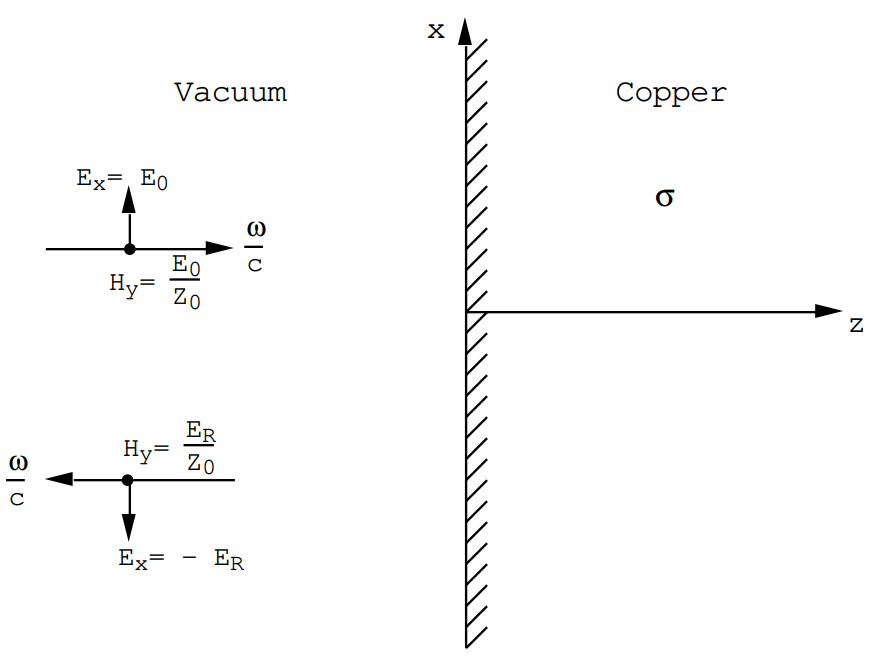
Considera un bloque de material dieléctrico de espesor d sumergido en vacío. Una onda que tiene una amplitud E _o es incidente en el bloque como se muestra: el ángulo de incidencia es θ = 0.

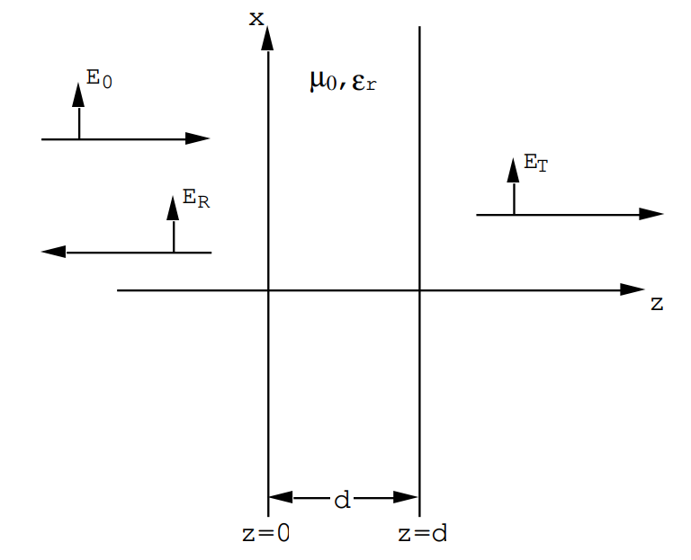
Calcular las amplitudes de las ondas reflejadas y transmitidas E _R, E _T.

CONSEJO: Dentro del bloque dieléctrico hay una onda que se mueve tanto hacia adelante como hacia atrás: es decir, en el bloque

\[E_{x}=a e^{i[k m z-\omega t]}+b e^{-i[k m z+\omega t]}\nonumber\]

Se deben cumplir las condiciones de contorno tanto en z = 0 como en z = d.

Respuesta (10.12).

En el bloque dieléctrico\(\mathrm{k}_{\mathrm{m}}^{2}=\varepsilon_{\mathrm{r}}\left(\frac{\omega}{\mathrm{c}}\right)^{2}\)

\(\therefore \mathrm{k}_{\mathrm{m}}=(\mathrm{n}+\mathrm{ik})\left(\frac{\omega}{\mathrm{c}}\right)\)si ε _r es complejo.

Requerimos rizo E = iωµ _o H

⟩ ya que solo hay un componente x de E

\[\mathrm{i} \omega \mu_{\circ} \mathrm{H}_{\mathrm{Y}}=\frac{\partial \mathrm{E}_{\mathrm{X}}}{\partial \mathrm{z}}=\mathrm{i} \mathrm{k}_{\mathrm{m}}\left[\mathrm{a} \mathrm{e}^{\mathrm{i}[\mathrm{kmz}-\omega \mathrm{t}]}-\mathrm{b} \mathrm{e}^{-\mathrm{i}[\mathrm{kmz}+\omega \mathrm{t}]}\right]\nonumber\]

Ola Incidente:

\[E_{x}=E_{0} e^{i[\omega / c \ z-\omega t]}\nonumber\]

\[\mathrm{H}_{\mathrm{y}}=\frac{\mathrm{E}_{\mathrm{0}}}{\mathrm{Z}_{\mathrm{0}}} e^{\mathrm{i}[\omega / \mathrm{c} \ \mathrm{z}-\omega \mathrm{t}]}\nonumber\]

Onda reflejada:

\[E_{x}=E_{R} e^{-i[\omega / c \ z+\omega t]}\nonumber\]

\[\mathrm{H}_{\mathrm{Y}}=-\frac{\mathrm{E}_{\mathrm{R}}}{\mathrm{Z}_{\mathrm{0}}} e^{-\mathrm{i}[\omega / \mathrm{c} \ \mathrm{z}+\omega \mathrm{t}]}\nonumber\]

Condiciones de contorno en z = 0

(1) Continuidad de E _x\(\mathbf{E}_{\mathbf{0}}+\mathbf{E}_{\mathbf{R}}=\mathbf{a}+\mathbf{b} \quad \quad \quad \quad (1) \)

(2) Continuidad de H _y\( \frac{E_{0}}{Z_{0}}-\frac{E_{R}}{Z_{0}}=\frac{c k_{m}}{\omega Z_{0}}[a-b]\)

o\(\mathbf{E}_{0}-\mathbf{E}_{R}=\frac{\mathbf{c} \mathbf{k}_{m}}{\omega}[\mathbf{a}-\mathbf{b}] \quad \quad \quad \quad (2) \) (2)

Ahora en z = d uno puede escribir los campos transmitidos como

\[\left.E_{x}=E_{T} e^{i[\omega / c \ (z-d)}-\omega t\right]\nonumber\]

\[\mathrm{H}_{\mathrm{y}}=\frac{\mathrm{E}_{\mathrm{T}}}{\mathrm{Z}_{\mathrm{0}}} e^{\mathrm{i}[\omega / \mathrm{c} \ (\mathrm{z}-\mathrm{d})-\omega \mathrm{t}]}\nonumber\]

* en z = d E _x = E _T y H _y = E _T /Z _o

Pero en el dieléctrico a z = d uno tiene

\[E_{x}=\left(a e^{i k_m d} +b e^{-i k_m d}\right) e^{-i \omega t}\nonumber\]

\[\mathrm{H}_{\mathrm{Y}}=\frac{\mathrm{ck}_{\mathrm{m}}}{\omega \mathrm{Z}_{\mathrm{0}}} \left(a_{\mathrm{b}} e^{\mathrm{i} \mathrm{k_m} \mathrm{d}}-\mathrm{b} e^{-\mathrm{i} \mathrm{k_m} \mathrm{d}}\right) \mathrm{e}^{-\mathrm{i} \omega \mathrm{t}}\nonumber\]

Por lo tanto a partir de la continuidad de E _x se obtiene

\(\mathrm{a} \mathrm{e}^{\mathrm{i} \mathbf{k_m} \mathrm{d}}+\mathrm{b} \mathrm{e}^{-\mathrm{i} \mathbf{k_m} \mathrm{d}}=\mathrm{E}_{\mathrm{T}}\)(1)

y de continuidad de H _y

\[\frac{c k_{m}}{\omega Z_{0}}\left(a e^{i k_m d}-b e^{-i k_m d}\right)=\frac{E_{T}}{Z_{0}}\nonumber\]

o

\(\mathbf{a} e^{\mathbf{i} \mathbf{k_m} \mathbf{d}}-\mathbf{b} e^{-\mathbf{i} \mathbf{k_m} \mathbf{d}}=\left(\frac{\omega}{\mathbf{c} \mathbf{k}_{\mathrm{m}}}\right) \mathbf{E}_{\mathbf{T}}\nonumber\)(4)

De (3) y (4) uno tiene

\(\mathrm{a} \mathrm{e}^{\mathrm{i} \mathrm{k_m} \mathrm{d}}-\mathrm{b} \mathrm{e}^{-\mathrm{i} \mathrm{k_m} \mathrm{d}}=\left(\frac{\omega}{\mathrm{ck}_{\mathrm{m}}}\right)\left[\mathrm{a} \mathrm{e}^{\mathrm{i} \mathrm{k_m} \mathrm{d}}+\mathrm{b} \mathrm{e}^{-\mathrm{i} \mathrm{k_md}}\right]\)

\(\therefore \quad \frac{\mathrm{b}}{\mathrm{a}}=\mathrm{e}^{2 \mathrm{i} \mathrm{k_m} \mathrm{d}}\left[\frac{1-\left(\frac{\omega}{\mathrm{ck}_{\mathrm{m}}}\right)}{1+\left(\frac{\omega}{\mathrm{ck}_{\mathrm{m}}}\right)}\right]\)

y de (1) y (2)

\(2 \mathrm{E}_{\mathrm{0}}=\mathrm{a}\left\{\left[1+\left(\frac{\mathrm{ck}_{\mathrm{m}}}{\omega}\right)\right]+\left[1-\left(\frac{\mathrm{c} \mathrm{k}_{\mathrm{m}}}{\omega}\right)\right]\left(\frac{\mathrm{b}}{\mathrm{a}}\right)\right\}\)

o

\[\frac{\mathrm{a}}{\mathrm{E}_{\mathrm{o}}}=\frac{2\left(1+\frac{\omega}{\mathrm{ck}_{\mathrm{m}}}\right)}{\left[\left(2+\frac{\omega}{\mathrm{ck}_{\mathrm{m}}}+\frac{\mathrm{ck}_{\mathrm{m}}}{\omega}\right)+\left(2-\frac{\omega}{\mathrm{ck}_{\mathrm{m}}}-\frac{\mathrm{ck}_{\mathrm{m}}}{\omega}\right) \mathrm{e}^{2 \mathrm{i} \mathrm{k_m} \mathrm{d}}\right]}\nonumber\]

\[\frac{\mathbf{b}}{\mathbf{E}_{\mathrm{O}}}=\frac{2\left(1-\frac{\omega}{\mathbf{c} \mathbf{k}_{\mathrm{m}}}\right)}{\left[\left(2+\frac{\omega}{\mathbf{c} \mathbf{k}_{\mathrm{m}}}+\frac{\mathbf{c} \mathbf{k}_{\mathrm{m}}}{\omega}\right)+\left(2-\frac{\omega}{\mathbf{c} \mathbf{k}_{\mathrm{m}}}-\frac{\mathbf{c} \mathbf{k}_{\mathrm{m}}}{\omega}\right) \mathrm{e}^{2 \mathbf{i} \mathbf{k}_{\mathrm{m}} \mathrm{d}}\right]}\nonumber\]

\[\frac{E_{R}}{E_{0}}=\frac{\left[\left(\frac{\omega}{c k_{m}}\right)-\left(\frac{c k_{m}}{\omega}\right)\right]\left[1-e^{2 i k_m d}\right]}{\left[\left(2+\frac{\omega}{c k_{m}}+\frac{c k_{m}}{\omega}\right)+\left(2-\frac{\omega}{c k_{m}}-\frac{c k_{m}}{\omega}\right) e^{2 i k_m d}\right]}\nonumber\]

\[\frac{E_{T}}{E_{0}}=\frac{4 e^{i k_m d}}{\left[\left(2+\frac{\omega}{c k_{m}}+\frac{c k_{m}}{\omega}\right)+\left(2-\frac{\omega}{c k_{m}}-\frac{c k_{m}}{\omega}\right) e^{2 i k_m d}\right]}\nonumber\]

Si ε _r es real k _m = nω/c y

\(\left(\frac{E_{R}}{E_{0}}\right)=\frac{\left(1-n^{2}\right)\left[1-e^{2 i k_m d}\right]}{\left[(n+1)^{2}-(n-1) 2 e^{2 i k_m d}\right]}\)

\(\left(\frac{E_{T}}{E_{0}}\right)=\frac{4 n e^{i k_m d}}{\left[(n+1) 2-(n-1) 2 e^{2 i k_m d}\right]}\)

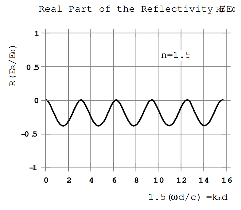
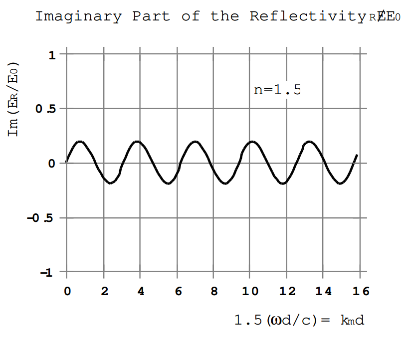
Las dos ecuaciones anteriores son funciones oscilatorias de la longitud de onda.

si 2k _m d = 2\(\pi\), 4\(\pi\), 6\(\pi\), etc.

entonces\(\frac{E_{R}}{E_{0}}=0\)\(\frac{E_{T}}{E_{0}}=\pm 1\)

Si 2k _m d =\(\pi\), 3\(\pi\), 5\(\pi\), etc.

entonces\(\frac{E_{R}}{E_{0}}=\frac{\left(1-n^{2}\right)}{\left(1+n^{2}\right)}\) es decir, un máximo

\(\frac{E_{T}}{E_{0}}=\frac{\pm 2 n i}{\left(n^{2}+1\right)}\)

La variación con frecuencia de la reflectividad y el coeficiente de transmisión se trazan a continuación para una constante dieléctrica real ε _r = 2.25 (n= 1.5).

Problema (10.13).

Que se describa un material por respuesta lineal eléctrica y magnética: i.e.

\[\mathbf{D}=\varepsilon(\omega) \mathbf{E},\nonumber\]

y

\[\mathbf{B}=\boldsymbol{\mu}(\boldsymbol{\omega}) \mathbf{H},\nonumber\]

donde tanto ε (ω) como µ (ω) son números complejos. Estos suelen estar escritos

\[\varepsilon(\omega)=\varepsilon_{0} \varepsilon_{r}=\varepsilon_{1}+i \varepsilon_{2}\nonumber\]

y

\[\mu(\omega)=\mu_{0} \mu_{r}=\mu_{1}+\mu_{2}.\nonumber\]

Para una dependencia\(e^{-i \omega t}\) del tiempo las partes imaginarias de las funciones de respuesta, ε ₂ (ω) y µ ₂ (ω), son mayores que cero.

(a) Según el teorema de Poynting, la tasa de incremento de la energía almacenada en los campos viene dada por

\[\frac{d W}{d t}=\mathbf{E} \cdot \frac{d \mathbf{D}}{d t}+\mathbf{H} \cdot \frac{d \mathbf{B}}{d t}.\nonumber\]

Mostrar que para una dependencia de tiempo\(e^{-i \omega t}\) las partes imaginarias de ε y µ deben ser mayores que cero para cualquier frecuencia finita. Esta conclusión se desprende de la restricción de que el promedio de tiempo de\(\frac{d W}{d t}\) debe ser mayor o igual a cero según la segunda ley de la termodinámica.

(b) Demostrar que para\(e^{-i \omega t}\) una dependencia del tiempo se puede encontrar una solución de onda plana de las ecuaciones de Maxwell en la forma

\[E_{x}=E_{0} e^{i\left(k_{m} z-\omega t\right)} \quad \quad \quad \quad (1) \nonumber\]

\[\mathrm{H}_{\mathrm{Y}}=\frac{\mathrm{k}_{\mathrm{m}}}{\omega \mu} \mathrm{E}_{0} \mathrm{e}^{\mathrm{i}\left(\mathrm{k}_{\mathrm{m}} \mathrm{z}-\omega \mathrm{t}\right)}, \quad \quad \quad \quad (2)\nonumber\]

donde\(\mathrm{k}_{\mathrm{m}}^{2}=\varepsilon_{\mathrm{r}} \mu_{\mathrm{r}}\left(\frac{\omega}{\mathrm{c}}\right)^{2},\)

y\(\mathrm{k}_{\mathrm{m}}=\sqrt{\varepsilon_{\mathrm{r}} \mu_{\mathrm{r}}}\left(\frac{\omega}{\mathrm{c}}\right) \equiv(\mathrm{N}+\mathrm{i} \kappa)\left(\frac{\omega}{\mathrm{c}}\right)\), donde K>0

para una ola amortiguada hacia el interior de una losa semi-infinita.

(c) Calcular el valor promedio de tiempo del vector Poynting correspondiente a los campos de eqns. (1) y (2). Demostrar que

\(\left\langle S_{z}\right\rangle=\frac{1}{2 C} \frac{\left(N \mu_{1}+K \mu_{2}\right)}{\left(\mu_{1}^{2}+\mu_{2}^{2}\right)}\left|E_{0}\right|^{2} e^{-2 \kappa\left(\frac{\omega}{c}\right) z}.\)(3)

Observe que para un medio pasivo <S _z > debe ser mayor que, o igual, a cero; esto significa que\(\left(\mathrm{N} \mu_{1}+\mathrm{K} \mu_{2}\right) \geq 0\). Para un material no magnético µ ₁ = µ ₀ y µ ₂ =0; así para un material no magnético eqn. (3) establece que n≥ 0 (para este caso n=N).

(d) Calcular las densidades de energía promediadas en el tiempo correspondientes a las ondas de eqns. (1) y (2). Demostrar que

\(<W_{E}>=\frac{1}{2} \operatorname{Real}\left(\frac{\varepsilon E E^{*}}{2}\right)=\frac{\varepsilon_{1}\left|E_{0}\right|^{2}}{4} e^{-2 K\left(\frac{\omega}{c}\right) z},\)(4)

y

\(<\mathrm{W}_{\mathrm{B}}>=\frac{1}{2} \operatorname{Real}\left(\frac{\mu \mathrm{HH}^{*}}{2}\right)=\frac{\varepsilon_{0} \mu_{0}}{4}\left(\frac{\mu_{1}}{\mu_{1}^{2}+\mu_{2}^{2}}\right)\left(\mathrm{N}^{2}+\mathrm{K}^{2}\right)\left|\mathrm{E}_{0}\right|^{2} \mathrm{e}^{-2 \mathrm{K}\left(\frac{\omega}{\mathrm{c}}\right) \mathrm{z}}\)(5)

Las expresiones (4) y (5) no parecen tener mucho en común excepto el factor\(\left|E_{0}\right|^{2} e^{-2 K\left(\frac{\omega}{c}\right) z}\). Sin embargo, a partir de la definición

\[\left(\varepsilon_{1}+i \varepsilon_{2}\right)\left(\mu_{1}+i \mu_{2}\right) \equiv(N+i K)^{2} \varepsilon_{0} \mu_{0}\nonumber\]

más algunos álgebra tediosa, se puede demostrar que

\(\varepsilon_{1}=\left(\frac{\left(\mathrm{N}^{2}-\mathrm{K}^{2}\right) \mu_{1}+2 \mathrm{NK} \mu_{2}}{\left(\mu_{1}^{2}+\mu_{2}^{2}\right)}\right) \varepsilon_{0} \mu_{0}\), (6)

y

\(\varepsilon_{2}=\left(\frac{2 \mathrm{NK} \boldsymbol{\mu}_{1}-\left(\mathrm{N}^{2}-\mathrm{K}^{2}\right) \mu_{2}}{\left(\mu_{1}^{2}+\mu_{2}^{2}\right)}\right) \varepsilon_{0} \mu_{0}.\)(7)

Estos se pueden utilizar para escribir

\(<\mathrm{W}_{\mathrm{E}}>=\frac{\varepsilon_{0} \mu_{0}}{4}\left(\frac{\left(\mathrm{N}^{2}-\mathrm{K}^{2}\right) \mu_{1}+2 \mathrm{NK} \mu_{2}}{\left(\mu_{1}^{2}+\mu_{2}^{2}\right)}\right)\left|\mathrm{E}_{0}\right|^{2} \mathrm{e}^{-2 \mathrm{K}\left(\frac{\omega}{\mathrm{c}}\right) \mathrm{z}}.\)(8)

(e) Calcular la densidad de energía promediada en el tiempo total asociada a los campos eléctricos y magnéticos de los eqns. (1) y (2). Demostrar que ya que\(<W>=\left\langle W_{E}\right\rangle+\left\langle W_{B}\right\rangle\) se deduce que

\(<\mathrm{W}>=\frac{\varepsilon_{0} \mu_{0}}{2} \frac{\mathrm{N}\left(\mathrm{N} \mu_{1}+\mathrm{K} \mu_{2}\right)}{\left(\mu_{1}^{2}+\mu_{2}^{2}\right)}\left|\mathrm{E}_{0}\right|^{2} e^{-2 \mathrm{K}\left(\frac{\omega}{\mathrm{c}}\right) \mathrm{z}}.\)(9)

Si esta densidad de energía va a ser no negativa, se deduce de eqn. (3) para <S _z > que debe ser mayor o igual a cero, que N≥0. Por comparación de eqns. (3) y (9) se encuentra también que

\[<S_{z}>=\left(\frac{c}{N}\right)<W>.\nonumber\]

No conozco ninguna razón microscópica fundamental por la que la parte real del índice de refracción deba limitarse a valores positivos. Es cierto, sin embargo, que para los metales que he comprobado, Fe, Co, Ni, Cu, Ag, Au y Al, la parte real del índice de refracción, n, es mayor que cero sobre el rango de energía 0.1 a 100 eV. Por ejemplo,

(i) Cu: n es un mínimo a 1.80 eV donde n=0.21 y\(\kappa\) =4.25; el índice luego aumenta con la energía pero se vuelve menor a 1 para energías mayores a 9.0 eV.

(ii) Ag: n es un mínimo a 3.5 eV donde n=0.21 y\(\kappa\) =1.42; el índice luego aumenta con la energía y vuelve a ser menor de 1 para energías mayores a 25 eV.

(iii) Au: n es un mínimo a 1.40 eV donde n=0.08 y\(\kappa\) =5.44; el índice luego aumenta con la energía pero se vuelve menor a 1 para energías mayores a 22 eV.

(iv) Al: n es un mínimo a 12.0 eV donde n=0.033 y\(\kappa\) =5.44; el índice luego aumenta con la energía pero cae por debajo de 1 para energías mayores a 95 eV.

Respuesta (10.13).

(a) Dejar\(E_{x}=E_{0} e^{-i \omega t}=E_{0} \cos \omega t\)

entonces\(D_{\mathrm{X}}=\left(\varepsilon_{1}+i \varepsilon_{2}\right) E_{0} e^{-i \omega t}\)

o

\[\mathrm{D}_{\mathrm{x}}=\varepsilon_{1} \mathrm{E}_{0} \mathrm{Cos} \omega \mathrm{t}+\varepsilon_{2} \mathrm{E}_{0} \operatorname{Sin} \omega \mathrm{t}.\nonumber\]

\[\frac{d W_{E}}{d t}=E_{x} \frac{d D_{x}}{d t}=E_{0} \cos \omega t\left(-\varepsilon_{1} \omega E_{0} \operatorname{Sin} \omega t+\varepsilon_{2} \omega E_{0} \cos \omega t\right),\nonumber\]

\[\frac{\mathrm{d} W_{\mathrm{E}}}{\mathrm{dt}}=-\omega \varepsilon_{1} \mathrm{E}_{0}^{2} \sin \omega \mathrm{t} \cos \omega \mathrm{t}+\omega \varepsilon_{2} \mathrm{E}_{0}^{2} \cos ^{2} \omega \mathrm{t}.\nonumber\]

Por lo tanto\(<\frac{d W_{E}}{d t}>=\omega \varepsilon_{2} \frac{E_{0}^{2}}{2}\).

De ello se deduce que si\(<\frac{d W_{E}}{d t}> \ \geq 0\) entonces\(\varepsilon_{2} \geq 0\) para cualquier frecuencia finita.

Del mismo modo\(\mathrm{H}_{\mathrm{y}}=\mathrm{H}_{0} \mathrm{e}^{-\mathrm{i} \omega \mathrm{t}}=\mathrm{H}_{0} \cos \omega \mathrm{t}\),

y\(\mathrm{B}_{\mathrm{y}}=\mu \mathrm{H}_{\mathrm{y}}=\mu_{1} \mathrm{H}_{0} \text { cos } \omega \mathrm{t}+\mu_{2} \mathrm{H}_{0} \sin \omega t\).

\[\frac{\mathrm{dB}_{\mathrm{Y}}}{\mathrm{dt}}=\omega \mathrm{H}_{0}\left(-\mu_{1} \sin \omega \mathrm{t}+\mu_{2} \cos \omega \mathrm{t}\right),\nonumber\]

por lo tanto

\[\frac{d W_{B}}{d t}=\mathbf{H} \cdot \frac{d \mathbf{B}}{d t}\nonumber\]

\[\frac{\mathrm{d} W_{B}}{d t}=\omega H_{0}^{2} \left(-\mu_{1} \sin \omega t \cos \omega t+\mu_{2} \cos ^{2} \omega t\right),\nonumber\]

y

\[<\frac{d W_{B}}{d t}>=\omega \mu_{2} \frac{H_{0}^{2}}{2}.\nonumber\]

De ello se deduce que si\(<\frac{d W_{B}}{d t}> \ \geq 0\) entonces\(\mu_{2} \geq 0\) para cualquier frecuencia finita.

(b) Las ecuaciones de Maxwell para una dependencia del tiempo\(e^{-i \omega t}\) pueden escribirse

\[\operatorname{curl} \mathbf{E}=\operatorname{i} \omega \mu \mathbf{H}=i \omega \mu_{r} \mu_{0} \mathbf{H} \quad \quad \quad \quad (i)\nonumber\]

\[\operatorname{curl} \mathbf{H}=-\mathrm{i} \omega \varepsilon \mathbf{E}=-\mathrm{i} \omega \varepsilon_{\mathrm{r}} \varepsilon_{0} \mathbf{E} \quad \quad \quad \quad (ii)\nonumber\]

donde de (i) div H =0 y de (ii) div E =0 porque la divergencia de cualquier curl debe desaparecer. Por lo tanto, los campos E, H satisfacen

\[\nabla^{2} \mathbf{E}=-\varepsilon_{\mathrm{r}} \mu_{\mathrm{r}}\left(\frac{\omega}{\mathrm{c}}\right)^{2} \mathbf{E}, \nonumber\]

\[\nabla^{2} \mathbf{H}=-\varepsilon_{\mathrm{r}} \mu_{\mathrm{r}}\left(\frac{\omega}{\mathrm{c}}\right)^{2} \mathrm{H}.\nonumber\]

Sea polarizado E a lo largo de x y H sea polarizado a lo largo de y Entonces las soluciones de onda plana de las ecuaciones anteriores son

\[E_{x}=E_{0} e^{i\left(k_{m} z-\omega t\right)}\nonumber\]

y

\[\mathrm{H}_{\mathrm{y}}=\mathrm{H}_{0} \mathrm{e}^{\mathrm{i}\left(\mathrm{k}_{\mathrm{m}} \mathrm{z}-\omega \mathrm{t}\right)}\nonumber\]

o

\[\mathrm{H}_{\mathrm{Y}}=\frac{\mathrm{k}_{\mathrm{m}}}{\omega \mu} \mathrm{E}_{0} \mathrm{e}^{\mathrm{i}\left(\mathrm{k}_{\mathrm{m}} \mathrm{z}-\omega \mathrm{t}\right)}, \text { from eqn. }(\mathrm{i}),\nonumber\]

donde\(\mathrm{k}_{\mathrm{m}}^{2}=\varepsilon_{\mathrm{r}} \mu_{\mathrm{r}}\left(\frac{\omega}{\mathrm{c}}\right)^{2}\)

o\(\mathrm{k}_{\mathrm{m}}=(\mathrm{N}+\mathrm{iK})\left(\frac{\omega}{\mathrm{c}}\right)\),

donde\(\mathrm{N}+\mathrm{i} \mathrm{K}=\sqrt{\varepsilon_{\mathrm{r}} \mu_{\mathrm{r}}}\).

Es necesario utilizar la rama de la raíz cuadrada para la cual K≥0, ya que esta rama corresponde a una perturbación que muere al aumentar z.

\[<\mathrm{S}_{\mathrm{z}}>=\frac{1}{2} \operatorname{Real}\left(\mathrm{E}_{\mathrm{x}} \mathrm{H}_{\mathrm{y}}^{*}\right),\nonumber\]

\[ <\mathrm{S}_{\mathrm{z}}>=\frac{1}{2} \operatorname{Real}\left(\mathrm{E}_{0} \mathrm{e}^{\mathrm{i} \mathrm{k}_{\mathrm{m}} \mathrm{z}} \frac{\mathrm{k}_{\mathrm{m}}^{*}}{\omega \mu^{*}} \mathrm{E}_{0}^{*} \mathrm{e}^{-\mathrm{i} \mathrm{k}_{\mathrm{m}}^{*} \mathrm{z}}\right)\nonumber\]

\[<\mathrm{S}_{\mathrm{z}}>=\frac{1}{2 \mathrm{c}} \operatorname{Real}\left(\frac{(\mathrm{N}-\mathrm{i} \mathrm{K})\left(\mu_{1}+\mathrm{i} \mu_{2}\right)}{\mu \mu^{*}}\left|\mathrm{E}_{0}\right|^{2} e^{-2 \mathrm{K}\left(\frac{\omega}{\mathrm{c}}\right) \mathrm{z}}\right), \nonumber\]

\[\left\langle\mathrm{S}_{\mathrm{z}}\right\rangle=\frac{1}{2 \mathrm{c}} \frac{\left(\mathrm{N} \mu_{1}+\mathrm{K} \mu_{2}\right)}{\left(\mu_{1}^{2}+\mu_{2}^{2}\right)}\left|\mathrm{E}_{0}\right|^{2} \mathrm{e}^{-2 \mathrm{K}\left(\frac{\omega}{\mathrm{c}}\right) \mathrm{z}}. \nonumber\]

d)\(\left\langle W_{E}\right\rangle=\left\langle\frac{\mathbf{E \cdot D}}{2}\right\rangle=\frac{1}{4} \operatorname{Real}\left(E_{x} D_{x}^{*}\right)\), o

\[\left\langle W_{E}\right\rangle=\frac{1}{4} \operatorname{Real}\left(E_{0} e^{i\left(k_{m} z-\omega t\right)}\left(\varepsilon_{1}-i \varepsilon_{2}\right) E_{0}^{*} e^{-i\left(k_{m}^{*} z-\omega t\right)}\right), \nonumber\]

\[ <W_{E}>=\frac{1}{4} \operatorname{Real}\left(\left(\varepsilon_{1}-i \varepsilon_{2}\right)\left|E_{0}\right|^{2} e^{i\left(k_{m}-k_{m}^{*}\right) z}\right).\nonumber\]

Pero\(\left(\mathrm{k}_{\mathrm{m}}-\mathrm{k}_{\mathrm{m}}^{*}\right)=2 \mathrm{i} \mathrm{K}\left(\frac{\omega}{\mathrm{c}}\right)\), por lo tanto

\[ <W_{E}>=\frac{\varepsilon_{1}}{4}\left|E_{0}\right|^2 e^{-2 K\left(\frac{\omega}{c}\right) z}.\nonumber\]

\[ <W_{B}>=<\frac{\mu H^{2}}{2}>,\nonumber\]

\[ <W_{B}>=\frac{1}{4} \operatorname{Real}\left(\frac{\left(\mu_{1}+i \mu_{2}\right)}{\omega^{2}} \frac{k_{m} k_{m}^{*}}{\mu \mu^{*}}\left|E_{0}\right|^2 e^{-2 K\left(\frac{\omega}{c}\right) z}\right).\nonumber\]

Pero\(\mathrm{k}_{\mathrm{m}} \mathrm{k}_{\mathrm{m}}^{*}=\left(\mathrm{N}^{2}+\mathrm{K}^{2}\right)\left(\frac{\omega}{\mathrm{c}}\right)^{2}\)

y\(\mu \mu^{*}=\left(\mu_{1}^{2}+\mu_{2}^{2}\right)\),

para que

\[<W_{B}>=\frac{1}{4 c^{2}} \frac{\mu_{1}\left(N^{2}+K^{2}\right)}{\left(\mu_{1}^{2}+\mu_{2}^{2}\right)}\left|E_{0}\right|^{2} e^{-2 K\left(\frac{\omega}{c}\right) z},\nonumber\]

donde\(c^{2}=1 / \varepsilon_{0} \mu_{0}\).

(e) Simplemente agregue juntos <W _E > y <W _B > y use eqn. (6) anterior para obtener

\[<\mathrm{W}>=\frac{\varepsilon_{0} \mu_{0}}{2} \frac{\mathrm{N}\left(\mathrm{N} \mu_{1}+\mathrm{K} \mu_{2}\right)}{\left(\mu_{1}^{2}+\mu_{2}^{2}\right)}\left|\mathrm{E}_{0}\right|^{2} \mathrm{e}^{-2 \mathrm{K}\left(\frac{\omega}{\mathrm{c}}\right) \mathrm{z}}. \quad \quad \quad \quad (9)\nonumber\]

Problema (10.14).

La radiación que tiene una frecuencia de 1 MHz cae a incidencia normal del vacío sobre una lámina gruesa de cobre. La lámina de cobre es paralela al plano x-y y la superficie de la lámina se encuentra en z=0. La resistividad del cobre es ρ= 2.0x10 ^-8 Ohm-metros a temperatura ambiente.

a) ¿Cuánta energía es absorbida por metro cuadrado por la lámina de cobre si la intensidad del campo eléctrico en la onda incidente es de 1 V/m?

b) ¿Cuál será la energía absorbida por m ² si la radiación incidente cae sobre la superficie con un ángulo de incidencia de 45°? Que la radiación incidente sea polarizada p.

Respuesta (10.14).

En el metal

\[\begin{aligned}\operatorname{curl} \mathbf{E}=& i \omega \mu_{0} \mathbf{H} \\ \operatorname{curl} \mathbf{H} &=\sigma \mathbf{E} \\ \operatorname{div} \mathbf{E} &=0 \\\operatorname{div} \mathbf{H} &=0 \end{aligned}\nonumber\]

por lo tanto

\[\operatorname{curl curl} \mathbf{H}=\mathbf{i} \omega \sigma \mu_{0} \mathbf{H}, \nonumber\]

y\(\text { curl curl } \mathbf{E}=\mathbf{i} \omega \sigma \mu_{0} \mathbf{E}, \nonumber\)

donde

\[ \mathrm{k}_{\mathrm{m}}^{2}=\mathrm{i} \omega \sigma \mu_{0}\nonumber, \]

o

\[\mathrm{k}_{\mathrm{m}}=\sqrt{\frac{\omega \mu_{0} \sigma}{2}}(1+\mathrm{i})=\frac{(1+\mathrm{i})}{\delta}.\nonumber\]

También\(\frac{\partial \mathrm{E}_{\mathrm{x}}}{\partial \mathrm{z}}=\mathrm{i} \omega \mu_{0} \mathrm{H}_{\mathrm{Y}}\)

o

\[ \mathrm{E}_{\mathrm{x}}=\left(\frac{\omega \mu_{0}}{\mathrm{k}_{\mathrm{m}}}\right) \mathrm{H}_{\mathrm{y}}=\left(\frac{\delta \omega}{\mathrm{c}}\right) \mu_{0} \mathrm{c} \frac{(1-\mathrm{i})}{2} \mathrm{H}_{\mathrm{Y}}.\nonumber\]

Para este problema ω = 2\(\pi\) x10 ⁶ radianes/seg

\(\frac{\omega}{c}=0.0209 / \mathrm{m}\)

\(\delta=\sqrt{\frac{2}{\omega \mu_{0} \sigma}}=0.71 \times 10^{-4} \ \mathrm{m}=71 \mathrm{\mu m}\)

y\(\frac{\delta \omega}{\mathrm{c}}=1.49 \times 10^{-6}\).

En la onda incidente E ₀ = 1 V/m, y\(\mathrm{H}_{0}=\frac{\mathrm{E}_{0}}{\mathrm{Z}_{0}}=2.65 \times 10^{-3}\) Amps/m.

Justo dentro de la superficie metálica\(\mathrm{H}_{\mathrm{T}} \cong 2 \mathrm{H}_{0}=5.31 \times 10^{-3}\) Amps/m.

Por lo tanto\(E_{x}=\left(1.49 \times 10^{-6}\right)(377) \frac{(1-i)}{2}\left(5.31 \times 10^{-3}\right)\)

\(E_{x}=\left(1.49 \times 10^{-6}\right)(1-i) \quad V / m\).

\(\left\langle S_{x}\right\rangle=\frac{1}{2} \operatorname{Real}\left(H_{y} E_{x}^{*}\right)\)

\(\left\langle S_{x}\right\rangle=\operatorname{Real}\left(\left(2 \cdot 65 \times 10^{-3}\right)\left(1 \cdot 49 \times 10^{-6}\right)(1+i)\right)\)

\(\left\langle S_{x}\right\rangle=3.95 \times 10^{-9} \text {Watts } / \mathrm{m}^{2}\).

b) La ola incidente viene dada por

\[ \mathrm{H}_{\mathrm{Y}}=\mathrm{H}_{0} \mathrm{e}^{\mathrm{iqx}} \mathrm{e}^{\mathrm{ikz}} e^{-\mathrm{i} \omega \mathrm{t}}\nonumber\]

\[\mathrm{E}_{\mathrm{x}}=\frac{\mathrm{Z}_{0} \mathrm{H}_{0}}{\sqrt{2}} \mathrm{e}^{\mathrm{iqx}} \mathrm{e}^{\mathrm{ikz}} \mathrm{e}^{-\mathrm{i} \omega \mathrm{t}}\nonumber\]

\[\mathrm{E}_{\mathrm{z}}=-\frac{\mathrm{Z}_{0} \mathrm{H}_{0}}{\sqrt{2}} e^{\mathrm{i} \mathrm{q} \mathrm{x}} e^{\mathrm{i} \mathrm{k} \mathrm{z}} e^{-\mathrm{i} \omega \mathrm{t}}. \nonumber\]

La onda reflejada viene dada por

\[ \mathrm{H}_{\mathrm{y}}=\mathrm{H}_{\mathrm{R}} \mathrm{e}^{-\mathrm{i} \mathrm{k} \mathrm{z}} e^{-\mathrm{i} \omega \mathrm{t}}\nonumber\]

\[ \mathrm{E}_{\mathrm{x}}=-\frac{\mathrm{Z}_{0} \mathrm{H}_{\mathrm{R}}}{\sqrt{2}} e^{\mathrm{i} q \mathrm{x}} e^{-\mathrm{i} \mathrm{k} z} e^{-\mathrm{i} \omega \mathrm{t}}\nonumber\]

\[ \mathrm{E}_{\mathrm{z}}=-\frac{\mathrm{Z}_{0} \mathrm{H}_{\mathrm{R}}}{\sqrt{2}} e^{\mathrm{i} q \mathrm{x}} e^{-\mathrm{i} \mathrm{k} z} e^{-\mathrm{i} \omega t}.\nonumber\]

En el metal\(-\nabla^{2} \mathbf{H}=i \omega \sigma \mu_{0} \mathbf{H}\)

por lo tanto

\[q^{2}+k_{m}^{2}=i \omega \sigma \mu_{0} \nonumber\]

\[q^{2}+k_{m}^{2}=\frac{i\left(4 \pi \times 10^{-7}\right)\left(2 \pi \times 10^{6}\right)}{2 \times 10^{-8}}=3.95 i \times 10^{8} / \mathrm{m}^{2}\nonumber\]

y

\[q=\frac{\omega}{\operatorname{c} \sqrt{2}}=0.0148 / \mathrm{m}, \quad \mathrm{i} . \mathrm{e} \cdot \mathrm{q}^{2}=2.18 \times 10^{-4} / \mathrm{m}^{2}.\nonumber\]

En otras palabras, q ² es completamente despreciable en comparación con\(\mathrm{k}_{\mathrm{m}}^{2}\). Esto es, a todos los efectos, el mismo problema que la parte a). La energía absorbida por la onda incidente será de 3.95x10 ^-9 vatios/m ². Para integridad, si

\(\mathrm{H}_{\mathrm{Y}}=\mathrm{H}_{\mathrm{T}} e^{iqx} e^{ik_{m}z}\), entonces\(\mathrm{E}_{\mathrm{x}}=-\frac{\mathrm{i} \mathrm{k}_{\mathrm{m}}}{\sigma} \mathrm{H}_{\mathrm{T}} \mathrm{e}^{\mathrm{i} \mathrm{q} \mathrm{x}} \mathrm{e}^{\mathrm{i} \mathrm{k}_{\mathrm{m}} \mathrm{z}}\), donde\(\mathrm{H}_{\mathrm{T}} \cong 2 / \mathrm{Z}_{0}\), y Z ₀ = cµ ₀.