11.6: Campos por Ley de Gauss

10.6.1 Ley de Gauss

La pulga de la subsección 10.3.2 tuvo una larga e ilustre carrera científica, y ahora vamos a retomar su historia donde la dejamos. Esta pulga, cuyo nombre es Gauss ⁹, ha derivado la ecuación\(E_\perp=2\pi k\sigma\) para el campo eléctrico muy cerca de una superficie cargada con densidad de carga\(\sigma\). A continuación describiremos dos mejoras que va a hacer a esa ecuación.

Primero, se da cuenta de que la ecuación no es tan útil como podría ser, porque sólo da la parte del campo debido a la superficie. Si hay otros cargos cerca, entonces sus campos se sumarán a este campo como vectores, y la ecuación no será cierta a menos que restemos cuidadosamente el campo de las otras cargas. Esto es especialmente problemático para ella porque el planeta en el que vive, conocido por razones oscuras como planeta Flatcat, está en sí mismo cargado eléctricamente, al igual que todas las pulgas —lo único que les evita flotar hacia el espacio exterior es que están cargadas negativamente, mientras que Flatcat lleva un carga positiva, por lo que son atraídos eléctricamente hacia ella. Cuando Gauss encontró la versión original de su ecuación, quiso demostrársela a sus escépticos colegas en el laboratorio, utilizando medidores de campo eléctrico y piezas cargadas de lámina metálica. Aunque configurara las medidas por control remoto, para que ella la carga en su propio cuerpo estuviera demasiado lejos para tener algún efecto, serían interrumpidos por el campo ambiental del planeta Flatcat. Finalmente, sin embargo, se dio cuenta de que podría mejorar su ecuación reescribiéndola de la siguiente manera:

\[\begin{equation*} E_{outward,\ on\ side\ 1}+E_{outward,\ on\ side\ 2} = 4\pi k\sigma . \end{equation*}\]

Lo complicado aquí es que “hacia afuera” significa algo diferente, dependiendo de qué lado del foil estemos. En el lado izquierdo, “hacia afuera” significa a la izquierda, mientras que en el lado derecho, “hacia afuera” es derecho. Una pieza de lámina metálica cargada positivamente tiene un campo que apunta hacia la izquierda en el lado izquierdo, y hacia la derecha en su lado derecho, por lo que las dos contribuciones de\(2\pi k\sigma\) son ambas positivas, y obtenemos\(4\pi k\sigma\). Por otra parte, supongamos que hay un campo creado por otras cargas, no por el foil cargado, que pasa a apuntar a la derecha. En el lado derecho, este campo creado externamente está en la misma dirección que el campo del foil, pero en el lado izquierdo, el campo reduce la fuerza del campo hacia la izquierda creado por la lámina. El incremento en un término de la ecuación equilibra la disminución en el otro término. ¡Esta nueva versión de la ecuación es así exactamente correcta independientemente de qué campos generados externamente estén presentes!

Su siguiente innovación comienza multiplicando la ecuación en ambos lados por el área,\(A\), de un lado de la lámina:

\[\begin{align*} \left(E_{outward,\ on\ side\ 1}+E_{outward,\ on\ side\ 2}\right)A &= 4\pi k\sigma A \\ \text{or} \\ E_{outward,\ on\ side\ 1}A+E_{outward,\ on\ side\ 2}A &= 4\pi kq , \\ \end{align*}\]

donde\(q\) esta la carga del foil. El motivo de esta modificación es que ahora puede hacer que todo sea más atractivo definiendo un nuevo vector, el vector de área A.

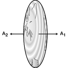
a / The area vector is defined to be perpendicular to the surface, in the outward direction. Its magnitude tells how much the area is.

As shown in figure a, she defines an area vector for side 1 which has magnitude \(A\) and points outward from side 1, and an area vector for side 2 which has the same magnitude and points outward from that side, which is in the opposite direction. The dot product of two vectors, \(\mathbf{u}\cdot\mathbf{v}\), can be interpreted as \(u_{parallel\ to\ v}|\mathbf{v}|\), and she can therefore rewrite her equation as

\[\begin{equation*} \mathbf{E}_1\cdot\mathbf{A}_1+\mathbf{E}_2\cdot\mathbf{A}_2 = 4\pi k q . \end{equation*}\]

The quantity on the left side of this equation is called the flux through the surface, written \(\Phi\).

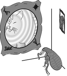
b / Gauss contemplates a map of the known world.

Gauss now writes a grant proposal to her favorite funding agency, the BSGS (Blood-Suckers' Geological Survey), and it is quickly approved. Her audacious plan is to send out exploring teams to chart the electric fields of the whole planet of Flatcat, and thereby determine the total electric charge of the planet. The fleas' world is commonly assumed to be a flat disk, and its size is known to be finite, since the sun passes behind it at sunset and comes back around on the other side at dawn. The most daring part of the plan is that it requires surveying not just the known side of the planet but the uncharted Far Side as well. No flea has ever actually gone around the edge and returned to tell the tale, but Gauss assures them that they won't fall off --- their negatively charged bodies will be attracted to the disk no matter which side they are on.

Of course it is possible that the electric charge of planet Flatcat is not perfectly uniform, but that isn't a problem. As discussed in subsection 10.3.2, as long as one is very close to the surface, the field only depends on the local charge density. In fact, a side-benefit of Gauss's program of exploration is that any such local irregularities will be mapped out. But what the newspapers find exciting is the idea that once all the teams get back from their voyages and tabulate their data, the total charge of the planet will have been determined for the first time. Each surveying team is assigned to visit a certain list of republics, duchies, city-states, and so on. They are to record each territory's electric field vector, as well as its area. Because the electric field may be nonuniform, the final equation for determining the planet's electric charge will have many terms, not just one for each side of the planet:

\[\begin{equation*} \Phi = \sum \mathbf{E}_j\cdot\mathbf{A}_j = 4\pi k q_{total} \end{equation*}\]

Gauss herself leads one of the expeditions, which heads due east, toward the distant Tail Kingdom, known only from fables and the occasional account from a caravan of traders. A strange thing happens, however. Gauss embarks from her college town in the wetlands of the Tongue Republic, travels straight east, passes right through the Tail Kingdom, and one day finds herself right back at home, all without ever seeing the edge of the world! What can have happened? All at once she realizes that the world isn't flat.

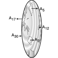
c / Each part of the surface has its own area vector. Note the differences in lengths of the vectors, corresponding to the unequal areas.

Now what? The surveying teams all return, the data are tabulated, and the result for the total charge of Flatcat is \((1/4\pi k)\sum \mathbf{E}_j\cdot\mathbf{A}_j=37\ \text{nC}\) (units of nanocoulombs). But the equation was derived under the assumption that Flatcat was a disk. If Flatcat is really round, then the result may be completely wrong. Gauss and two of her grad students go to their favorite bar, and decide to keep on ordering Bloody Marys until they either solve their problems or forget them. One student suggests that perhaps Flatcat really is a disk, but the edges are rounded. Maybe the surveying teams really did flip over the edge at some point, but just didn't realize it. Under this assumption, the original equation will be approximately valid, and 37 nC really is the total charge of Flatcat.

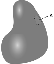
d / An area vector can be defined for a sufficiently small part of a curved surface.

A second student, named Newton, suggests that they take seriously the possibility that Flatcat is a sphere. In this scenario, their planet's surface is really curved, but the surveying teams just didn't notice the curvature, since they were close to the surface, and the surface was so big compared to them. They divided up the surface into a patchwork, and each patch was fairly small compared to the whole planet, so each patch was nearly flat. Since the patch is nearly flat, it makes sense to define an area vector that is perpendicular to it. In general, this is how we define the direction of an area vector, as shown in figure d. This only works if the areas are small. For instance, there would be no way to define an area vector for an entire sphere, since “outward” is in more than one direction.

If Flatcat is a sphere, then the inside of the sphere must be vast, and there is no way of knowing exactly how the charge is arranged below the surface. However, the survey teams all found that the electric field was approximately perpendicular to the surface everywhere, and that its strength didn't change very much from one location to another. The simplest explanation is that the charge is all concentrated in one small lump at the center of the sphere. They have no way of knowing if this is really the case, but it's a hypothesis that allows them to see how much their 37 nC result would change if they assumed a different geometry. Making this assumption, Newton performs the following simple computation on a napkin. The field at the surface is related to the charge at the center by

\[|\mathbf{E}| = \frac{kq_{total}}{r^2} ,\]

where \(r\) is the radius of Flatcat. The flux is then

\[ \Phi = \sum \mathbf{E}_j\cdot\mathbf{A}_j , \]

and since the \(\mathbf{E}_j\) and \(\mathbf{A}_j\) vectors are parallel, the dot product equals \(|\mathbf{E}_j||\mathbf{A}_j|\), so

\[\Phi = \sum \frac{kq_{total}}{r^2}|\mathbf{A}_j| .\]

But the field strength is always the same, so we can take it outside the sum, giving

\[\begin{align*} \Phi &= \frac{kq_{total}}{r^2} \sum |\mathbf{A}_j| \ &= \frac{kq_{total}}{r^2} A_{total} \ &= \frac{kq_{total}}{r^2} 4\pi r^2 \ &= 4\pi kq_{total} . \end{align*}\]

Not only have all the factors of \(r\) canceled out, but the result is the same as for a disk!

Everyone is pleasantly surprised by this apparent mathematical coincidence, but is it anything more than that? For instance, what if the charge wasn't concentrated at the center, but instead was evenly distributed throughout Flatcat's interior volume? Newton, however, is familiar with a result called the shell theorem (page 102), which states that the field of a uniformly charged sphere is the same as if all the charge had been concentrated at its center.¹⁰ We now have three different assumptions about the shape of Flatcat and the arrangement of the charges inside it, and all three lead to exactly the same mathematical result, \(\Phi = 4\pi kq_{total}\). This is starting to look like more than a coincidence. In fact, there is a general mathematical theorem, called Gauss' theorem, which states the following:

For any region of space, the flux through the surface equals \(4\pi kq_{in}\), where \(q_{in}\) is the total charge in that region.

Don't memorize the factor of \(4\pi\) in front --- you can rederive it any time you need to, by considering a spherical surface centered on a point charge.

Note that although region and its surface had a definite physical existence in our story --- they are the planet Flatcat and the surface of planet Flatcat --- Gauss' law is true for any region and surface we choose, and in general, the Gaussian surface has no direct physical significance. It's simply a computational tool.

Rather than proving Gauss' theorem and then presenting some examples and applications, it turns out to be easier to show some examples that demonstrate its salient properties. Having understood these properties, the proof becomes quite simple.

self-check:

Suppose we have a negative point charge, whose field points inward, and we pick a Gaussian surface which is a sphere centered on that charge. How does Gauss' theorem apply here?

(answer in the back of the PDF version of the book)

Contributors and Attributions

• Template:ContribCrowell