11.7: Ley de Gauss en forma diferencial

La ley de Gauss es un poco espeluznante. Se relaciona el campo en la superficie gaussiana con las cargas dentro de la superficie. ¿Y si los cargos se han ido moviendo, y el campo en la superficie ahora mismo es el que fue creado por los cargos en sus ubicaciones anteriores? La ley de Gauss —a diferencia de la ley de Coulomb— todavía funciona en casos como estos, pero está lejos de ser obvio cómo el flujo y los cargos pueden seguir estando de acuerdo si los cargos se han ido moviendo.

Por ello, sería más atractivo físicamente reafirmar la ley de Gauss en una forma diferente, de manera que relacionara el comportamiento del campo en un momento con los cargos que realmente estaban presentes en ese momento. Esto es esencialmente lo que estábamos haciendo en la fábula de la pulga llamada Gauss: el plan de las pulgas para vigilar su planeta era esencialmente uno de dividir la superficie de su planeta (que ellos creían que era plana) en un mosaico, y luego construir un pequeño pastillero gaussiano alrededor de cada parche pequeño. La ecuación\(E_{\perp}=2\pi k\sigma\) luego relacionó una propiedad particular del campo eléctrico local con la densidad de carga local.

En general, no es necesario que las distribuciones de carga se limiten a una superficie plana —la vida es tridimensional—, pero el enfoque general de definir superficies gaussianas muy pequeñas sigue siendo bueno. Nuestra estrategia es dividir el espacio en pequeños cubos, como el de la página 621. Cada uno de esos cubos constituye una superficie gaussiana, que puede contener alguna carga. Nuevamente aproximamos el campo usando sus seis valores en el centro de cada uno de los seis lados. Deje que el cubo se extienda de\(x\) a\(x+dx\), de\(y\) a\(y+dy\), y de\(y\) a\(y+dy\).

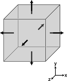
a / A tiny cubical Gaussian surface.

The sides at \(x\) and \(x+dx\) have area vectors \(-dydz\hat{\mathbf{x}}\) and \(dydz\hat{\mathbf{x}}\), respectively. The flux through the side at \(x\) is \(-E_x(x)dydz\), and the flux through the opposite side, at \(x+dx\) is \(E_x(x+dx)dydz\). The sum of these is \((E_x(x+dx)-E_x(x))dydz\), and if the field was uniform, the flux through these two opposite sides would be zero. It will only be zero if the field's \(x\) component changes as a function of \(x\). The difference \(E_x(x+dx)-E_x(x)\) can be rewritten as \(dE_x=(dE_x)/(dx)dx\), so the contribution to the flux from these two sides of the cube ends up being

\[\begin{equation*} \frac{dE_x}{dx}dxdydz . \end{equation*}\]

Doing the same for the other sides, we end up with a total flux

\[\begin{align*} d \Phi &= \left(\frac{dE_x}{dx}+\frac{dE_y}{dy} +\frac{dE_z}{dz}\right)dxdydz \\ &= \left(\frac{dE_x}{dx}+\frac{dE_y}{dy} +\frac{dE_z}{dz}\right)dv ,\end{align*}\]

where \(dv\) is the volume of the cube. In evaluating each of these three derivatives, we are going to treat the other two variables as constants, to emphasize this we use the partial derivative notation \(\partial\) introduced in chapter 3,

\[\begin{align*} d \Phi &= \left(\frac{\partial E_x}{\partial x}+\frac{\partial E_y}{\partial y} +\frac{\partial E_z}{\partial z}\right)dv .\\ \text{Using Gauss' law,} \\ 4\pi k q_{in} &= \left(\frac{\partial E_x}{\partial x}+\frac{\partial E_y}{\partial y} +\frac{\partial E_z}{\partial z}\right)dv ,\end{align*}\]

and we introduce the notation \(\rho\) (Greek letter rho) for the charge per unit volume, giving

\[\begin{align*} 4\pi k \rho &= \frac{\partial E_x}{\partial x}+\frac{\partial E_y}{\partial y} +\frac{\partial E_z}{\partial z} . \end{align*}\]

The quantity on the right is called the divergence of the electric field, written \(\rm div \mathbf{E}\). Using this notation, we have \(\rm div \mathbf{E} = 4\pi k \rho .\)

This equation has all the same physical implications as Gauss' law. After all, we proved Gauss' law by breaking down space into little cubes like this. We therefore refer to it as the differential form of Gauss' law, as opposed to \(\Phi=4\pi kq_{in}\), which is called the integral form.

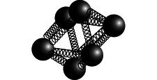
b / A meter for measuring \(\rm div \mathbf{E}\).

Figure b shows an intuitive way of visualizing the meaning of the divergence. The meter consists of some electrically charged balls connected by springs. If the divergence is positive, then the whole cluster will expand, and it will contract its volume if it is placed at a point where the field has \(\rm div \mathbf{E}\lt0\). What if the field is constant? We know based on the definition of the divergence that we should have \(\rm div \mathbf{E}=0\) in this case, and the meter does give the right result: all the balls will feel a force in the same direction, but they will neither expand nor contract.

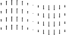
Example 36: Divergence of a sine wave

c / Example 36. \(\triangleright\) Figure c shows an electric field that varies as a sine wave. This is in fact what you'd see in a light wave: light is a wave pattern made of electric and magnetic fields. (The magnetic field would look similar, but would be in a plane perpendicular to the page.) What is the divergence of such a field, and what is the physical significance of the result? \(\triangleright\) Intuitively, we can see that no matter where we put the div-meter in this field, it will neither expand nor contract. For instance, if we put it at the center of the figure, it will start spinning, but that's it. Mathematically, let the \(x\) axis be to the right and let \(y\) be up. The field is of the form \[\begin{equation*} \mathbf{E} = (\text{sin} Kx)\: \hat{\mathbf{y}} , \end{equation*}\] where the constant \(K\) is not to be confused with Coulomb's constant. Since the field has only a \(y\) component, the only term in the divergence we need to evaluate is \[\begin{equation*} \mathbf{E} = \frac{\partial E_{y}}{\partial y} , \end{equation*}\] but this vanishes, because \(E_y\) depends only on \(x\), not \(y\) : we treat \(y\) as a constant when evaluating the partial derivative \(\partial E_{y}/\partial y\), and the derivative of an expression containing only constants must be zero. Physically this is a very important result: it tells us that a light wave can exist without any charges along the way to “keep it going.” In other words, light can travel through a vacuum, a region with no particles in it. If this wasn't true, we'd be dead, because the sun's light wouldn't be able to get to us through millions of kilometers of empty space!

Example 37: Electric field of a point charge

The case of a point charge is tricky, because the field behaves badly right on top of the charge, blowing up and becoming discontinuous. At this point, we cannot use the component form of the divergence, since none of the derivatives are well defined. However, a little visualization using the original definition of the divergence will quickly convince us that div \(E\) is infinite here, and that makes sense, because the density of charge has to be infinite at a point where there is a zero-size point of charge (finite charge in zero volume). At all other points, we have \[\begin{equation*} \mathbf{E} = \frac{ kq}{ r^2}\hat{\mathbf{r}} , \end{equation*}\] where \(\hat{\mathbf{r}}=\mathbf{r}/ r=( x\hat{\mathbf{x}}+ y\hat{\mathbf{y}}+ z\hat{\mathbf{z}})/ r\) is the unit vector pointing radially away from the charge. The field can therefore be written as \[\begin{align*} \mathbf{E} &= \frac{ kq}{ r^3}\hat{\mathbf{r}} \\ &= \frac{ kq( x\hat{\mathbf{x}}+ y\hat{\mathbf{y}}+ z\hat{\mathbf{z}})}{\left( x^2+ y^2+ z^2\right)^\text{3/2}} . \\ \text{The three terms in the divergence are all similar, e.g.,}\\ \frac{\partial E_{x}}{\partial x} &= kq\frac{\partial}{\partial x}\left[\frac{ x}{\left( x^2+ y^2+ z^2\right)^\text{3/2}}\right] \\ &= kq\left[\frac{1}{\left( x^2+ y^2+ z^2\right)^\text{3/2}}-\frac{3}{2}\:\frac{2 x^2}{\left( x^2+ y^2+ z^2\right)^\text{5/2}}\right] \\ &= kq\left( r^{-3}-3 x^2 r^{-5}\right) . \end{align*}\] Straightforward algebra shows that adding in the other two terms results in zero, which makes sense, because there is no charge except at the origin.

Gauss' law in differential form lends itself most easily to finding the charge density when we are give the field. What if we want to find the field given the charge density? As demonstrated in the following example, one technique that often works is to guess the general form of the field based on experience or physical intuition, and then try to use Gauss' law to find what specific version of that general form will be a solution.

Example 38: The field inside a uniform sphere of charge

\(\triangleright\) Find the field inside a uniform sphere of charge whose charge density is \(\rho\). (This is very much like finding the gravitational field at some depth below the surface of the earth.) \(\triangleright\) By symmetry we know that the field must be purely radial (in and out). We guess that the solution might be of the form \[\begin{equation*} \mathbf{E} = br^ p\hat{\mathbf{r}} , \end{equation*}\] where \(r\) is the distance from the center, and \(b\) and \(p\) are constants. A negative value of \(p\) would indicate a field that was strongest at the center, while a positive \(p\) would give zero field at the center and stronger fields farther out. Physically, we know by symmetry that the field is zero at the center, so we expect \(p\) to be positive. As in the example 37, we rewrite \(\hat{\mathbf{r}}\) as \(\mathbf{r}/ r\), and to simplify the writing we define \(n= p-1\), so \[\begin{equation*} \mathbf{E} = br^ n\mathbf{r} . \end{equation*}\] Gauss' law in differential form is \[\begin{equation*} \rm div \mathbf{E} = 4\pi k\rho , \end{equation*}\] so we want a field whose divergence is constant. For a field of the form we guessed, the divergence has terms in it like \[\begin{align*} \frac{\partial E_{x}}{\partial x} &= \frac{\partial}{\partial x}\left( br^{n} x\right) \\ &= b\left( nr^{ n-1}\frac{\partial r}{\partial x} x+r^ n\right) \\ \end{align*}\] The partial derivative \(\partial r/\partial x\) is easily calculated to be \(x/ r\), so \[\begin{equation*} \frac{\partial E_{x}}{\partial x} = b\left( nr^{ n-2} x^2+r^ n\right) \end{equation*}\] Adding in similar expressions for the other two terms in the divergence, and making use of \(x^2+ y^2+ z^2= r^2\), we have \[\begin{equation*} \rm div \mathbf{E} = b( n+3) r^ n . \end{equation*}\] This can indeed be constant, but only if \(n\) is 0 or \(-3\), i.e., \(p\) is 1 or \(-2\). The second solution gives a divergence which is constant and zero : this is the solution for the outside of the sphere! The first solution, which has the field directly proportional to \(r\), must be the one that applies to the inside of the sphere, which is what we care about right now. Equating the coefficient in front to the one in Gauss' law, the field is \[\begin{equation*} \mathbf{E} = \frac{4\pi k\rho}{3} r\:\hat{\mathbf{r}} . \end{equation*}\] The field is zero at the center, and gets stronger and stronger as we approach the surface.

Contributors and Attributions

Template:ContribCrowell