13.9: Trabajo realizado por una fuerza no constante a lo largo de un camino arbitrario

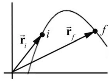
Supongamos que una fuerza no constante\(\overrightarrow{\mathbf{F}}\) actúa sobre un cuerpo de masa puntiforme m mientras el cuerpo se mueve en una trayectoria curva tridimensional. El vector de posición del cuerpo en el tiempo t con respecto a una elección de origen es\(\overrightarrow{\mathbf{r}}(t)\). En la Figura 13.15 se muestra la órbita del cuerpo por un intervalo de tiempo que\(\left[t_{i}, t_{f}\right]\) se mueve de una posición inicial\(\overrightarrow{\mathbf{r}}_{i} \equiv \overrightarrow{\mathbf{r}}\left(t=t_{i}\right)\) en el momento\(t=t_{i}\) a una posición final\(\overrightarrow{\mathbf{r}}_{f} \equiv \overrightarrow{\mathbf{r}}\left(t=t_{f}\right)\) en el momento\(t=t_{f}\).

Figura 13.15 Trayectoria trazada por el movimiento de un cuerpo.

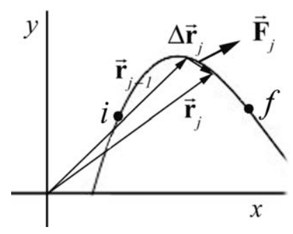
Dividimos el intervalo de tiempo\(\left[t_{i}, t_{f}\right]\) en N intervalos más pequeños con\(\left[t_{j-1}, t_{j}\right]\),\(j=1, \cdots, N\) con\(t_{N}=t_{f}\). Considere dos vectores de posición\(\overrightarrow{\mathbf{r}}_{j} \equiv \overrightarrow{\mathbf{r}}\left(t=t_{j}\right)\) y\(\overrightarrow{\mathbf{r}}_{j-1} \equiv \overrightarrow{\mathbf{r}}\left(t=t_{j-1}\right)\) el vector de desplazamiento durante el intervalo de tiempo correspondiente como\(\Delta \overrightarrow{\mathbf{r}}_{j}=\overrightarrow{\mathbf{r}}_{j}-\overrightarrow{\mathbf{r}}_{j-1}\). Dejar\(\overrightarrow{\mathbf{F}}\) denotar la fuerza que actúa sobre el cuerpo durante el intervalo\(\left[t_{j-1}, t_{j}\right]\). La fuerza promedio en este intervalo es\(\left(\overrightarrow{\mathbf{F}}_{j}\right)_{\mathrm{ave}}\) y el trabajo promedio\(\Delta W_{j}\) realizado por la fuerza durante el intervalo de tiempo\(\left[t_{j-1}, t_{j}\right]\) es el producto escalar entre el vector de fuerza promedio y el vector de desplazamiento,

\[\Delta W_{j}=\left(\overrightarrow{\mathbf{F}}_{j}\right)_{\mathrm{ave}} \cdot \Delta \overrightarrow{\mathbf{r}}_{j} \nonumber \]

La fuerza y los vectores de desplazamiento para el intervalo de tiempo se\(\left[t_{j-1}, t_{j}\right]\) muestran en la Figura 13.16 (obsérvese que el subíndice “ave” on\(\left(\overrightarrow{\mathbf{F}}_{j}\right)_{\mathrm{ave}}\) ha sido suprimido).

Figura 13.16 Un elemento de trabajo infinitesimal.

Calculamos el trabajo sumando estas contribuciones escalares al trabajo para cada intervalo\(\left[t_{j-1}, t_{j}\right]\), para j =1 a N,

\[W_{N}=\sum_{j=1}^{j=N} \Delta W_{j}=\sum_{j=1}^{j=N}\left(\overrightarrow{\mathbf{F}}_{j}\right)_{\mathrm{ave}} \cdot \Delta \overrightarrow{\mathbf{r}}_{j} \nonumber \]

Nos gustaría definir el trabajo de una manera que sea independiente de la forma en que dividimos el intervalo, así tomamos el límite como\(N \rightarrow \infty\) y\(\left|\Delta \overrightarrow{\mathbf{r}}_{j}\right| \rightarrow 0\) para todos j. En este límite, a medida que los intervalos se hacen cada vez más pequeños, la distinción entre la fuerza promedio y la fuerza real desaparece. Así, si este límite existe y está bien definido, entonces el trabajo realizado por la fuerza es

\[W=\lim _{N \rightarrow \infty \atop\left|\Delta \overrightarrow{\mathbf{r}}_{j}\right| \rightarrow 0} \sum_{j=1}^{j=N}\left(\overrightarrow{\mathbf{F}}_{j}\right)_{\text {ave }} \cdot \Delta \overrightarrow{\mathbf{r}}_{j}=\int_{i}^{f} \overrightarrow{\mathbf{F}} \cdot d \overrightarrow{\mathbf{r}} \nonumber \]

Observe que esta suma implica agregar cantidades escalares. A este límite se le llama la línea integral de la fuerza\(\overrightarrow{\mathbf{F}}\). El símbolo\(d \overrightarrow{\mathbf{r}}\) se llama el elemento de línea vectorial infinitesimal. En el tiempo t,\(d \overrightarrow{\mathbf{r}}\) es tangente a la órbita del cuerpo y es el límite del vector de desplazamiento a\(\Delta \overrightarrow{\mathbf{r}}=\overrightarrow{\mathbf{r}}(t+\Delta t)-\overrightarrow{\mathbf{r}}(t)\) medida que Δt se acerca a cero. En este límite, el parámetro t no aparece en la expresión en la Ecuación (13.8.19).

En general esta línea integral depende del camino particular que el cuerpo tome entre la posición inicial\(\overrightarrow{\mathbf{r}}_{i}\) y la posición final\(\overrightarrow{\mathbf{r}}_{f}\), lo que importa cuando la fuerza\(\overrightarrow{\mathbf{F}}\) es inconstante en el espacio, y cuando la contribución a la obra puede variar sobre diferentes caminos en el espacio. Podemos representar la integral en la Ecuación (13.8.19) explícitamente en un sistema de coordenadas especificando el elemento de línea vectorial infinitesimal d\(\overrightarrow{\mathbf{r}}\) y luego calculando explícitamente el producto escalar.

Trabajo Integral en Coordenadas Cartesianas

En las coordenadas cartesianas el elemento de línea es

\[d \overrightarrow{\mathbf{r}}=d x \hat{\mathbf{i}}+d y \hat{\mathbf{j}}+d z \hat{\mathbf{k}} \nonumber \]

donde dx, dy y dz representan desplazamientos arbitrarios en la\(\hat{\mathbf{k}}\) dirección\(\hat{\mathbf{i}}-, \hat{\mathbf{j}}-\), y -respectivamente, como se ve en la Figura 13.17.

Figura 13.17 Un elemento de línea en coordenadas cartesianas.

El vector de fuerza se puede representar en notación vectorial mediante

\[\overrightarrow{\mathbf{F}}=F_{x} \hat{\mathbf{i}}+F_{y} \hat{\mathbf{j}}+F_{z} \hat{\mathbf{k}} \nonumber \]

El trabajo infinitesimal es la suma del trabajo realizado por el componente de la fuerza multiplicado por el componente del desplazamiento en cada dirección,

\[d W=F_{x} d x+F_{y} d y+F_{z} d z \nonumber \]

La ecuación (13.8.22) es solo el producto escalar

\ [\ begin {alineado}
d W &=\ overrightarrow {\ mathbf {F}}\ cdot d\ overrightarrow {\ mathbf {r}} =\ left (F_ {x}\ hat {\ mathbf {i}} +F_ {y}\ hat {\ mathbf {j}} +F_ {z}\ sombrero {\ mathbf {k}} derecha)\ cdot (d x\ hat {\ mathbf {i}} +d y\ hat {\ mathbf {j}} +d z\ hat {\ mathbf {k}})\\
&=F_ {x} d x+f_ {y} d y+f_ {z} d z
\ end {alineado}\ nonumber\]

El trabajo es

\[W=\int_{\overrightarrow{\mathbf{r}}=\overrightarrow{\mathbf{r}}_{0}}^{\overrightarrow{\mathbf{r}}=\overrightarrow{\mathbf{r}}_{f}} \overrightarrow{\mathbf{F}} \cdot d \overrightarrow{\mathbf{r}}=\int_{\overrightarrow{\mathbf{r}}=\overrightarrow{\mathbf{r}}_{0}}^{\overrightarrow{\mathbf{r}}=\overrightarrow{\mathbf{r}}_{f}}\left(F_{x} d x+F_{y} d y+F_{z} d z\right)=\int_{\overrightarrow{\mathbf{r}}=\overrightarrow{\mathbf{r}}_{0}}^{\overrightarrow{\mathbf{r}}=\overrightarrow{\mathbf{r}}_{f}} F_{x} d x+\int_{\overrightarrow{\mathbf{r}}=\overrightarrow{\mathbf{r}}_{0}}^{\overrightarrow{\mathbf{r}}=\overrightarrow{\mathbf{r}}_{f}} \cdot \overrightarrow{d y+\int_{z=\overrightarrow{\mathbf{r}}_{0}}} F_{z} d z \nonumber \]

Trabajo Integral en Coordenadas Cilíndricas

En coordenadas cilíndricas el elemento de línea es

\[d \overrightarrow{\mathbf{r}}=d r \hat{\mathbf{r}}+r d \theta \hat{\mathbf{\theta}}+d z \hat{\mathbf{k}} \nonumber \]

donde dr, rdθ y dz representan desplazamientos arbitrarios en las\(\hat{\mathbf{k}}-\) direcciones\(\hat{\mathbf{r}}-, \hat{\boldsymbol{\theta}}-\) y respectivamente como se ve en la Figura 13.18.

Figura 13.18 Vector de desplazamiento\(d \overrightarrow{\mathbf{s}}\) entre dos puntos

El vector de fuerza se puede representar en notación vectorial mediante

\[\overrightarrow{\mathbf{F}}=F_{r} \hat{\mathbf{r}}+F_{\theta} \hat{\boldsymbol{\theta}}+F_{z} \hat{\mathbf{k}} \nonumber \]

El trabajo infinitesimal es el producto escalar

\ [\ begin {alineado}
d W &=\ overrightarrow {\ mathbf {F}}\ cdot d\ overrightarrow {\ mathbf {r}} =\ left (F_ {r}\ hat {\ mathbf {r}} +F_ {\ theta}\ hat {\ boldsymbol {\ theta} +F_ z {}\ hat {\ mathbf {k}}\ derecha)\ cdot (d r\ hat {\ mathbf {r}} +r d\ theta\ hat {\ boldsymbol {\ theta}} +d z\ hat {\ mathbf {k}})\\
&=F _ {r} d r+f_ {\ theta} r d\ theta+f_ {z} d z
\ final {alineado}\ nonumber\]

El trabajo es

\[W=\int_{\overrightarrow{\mathbf{r}}=\overrightarrow{\mathbf{r}}_{0}}^{\overrightarrow{\mathbf{r}}=\overrightarrow{\mathbf{r}}_{f}} \cdot \overrightarrow{\mathbf{r}}=\int_{\overrightarrow{\mathbf{r}}=\overrightarrow{\mathbf{r}}_{0}}^{\overrightarrow{\mathbf{r}}=\overrightarrow{\mathbf{r}}_{f}}\left(F_{r} d r+F_{\theta} r d \theta+F_{z} d z\right)=\int_{\overrightarrow{\mathbf{r}}=\overrightarrow{\mathbf{r}}_{0}}^{\overrightarrow{\mathbf{r}}=\overrightarrow{\mathbf{r}}_{f}} F_{r} d r+\int_{\overrightarrow{\mathbf{r}}=\overrightarrow{\mathbf{r}}_{0}}^{\overrightarrow{\mathbf{r}}=\overrightarrow{\mathbf{r}}_{f}} F_{\theta} r d \theta+\int_{\overrightarrow{\mathbf{r}}=\overrightarrow{\mathbf{r}}_{0}}^{\overrightarrow{\mathbf{r}}=\overrightarrow{\mathbf{r}}_{f}} F_{z} d z \nonumber \]