17.2: Producto vectorial (producto cruzado)

Dejar\(\overrightarrow{\mathbf{A}}\) y\(\overrightarrow{\mathbf{B}}\) ser dos vectores. Debido a que dos vectores no paralelos forman un plano, denotamos el ángulo θ para ser el ángulo entre los vectores\(\overrightarrow{\mathbf{A}}\) y\(\overrightarrow{\mathbf{B}}\) como se muestra en la Figura 17.2. La magnitud del vector producto\(\overrightarrow{\mathbf{A}} \times \overrightarrow{\mathbf{B}}\) de los vectores\(\overrightarrow{\mathbf{A}}\) y\(\overrightarrow{\mathbf{B}}\) se define como producto de la magnitud de los vectores\(\overrightarrow{\mathbf{A}}\) y\(\overrightarrow{\mathbf{B}}\) con el seno del ángulo θ entre los dos vectores,

\[|\overrightarrow{\mathbf{A}} \times \overrightarrow{\mathbf{B}}|=|\overrightarrow{\mathbf{A}}||\overrightarrow{\mathbf{B}}| \sin (\theta) \nonumber \]

El ángulo θ entre los vectores se limita a los valores que\(0 \leq \theta \leq \pi\) aseguran eso\(\sin (\theta) \geq 0\).

Figura 17.2 Geometría vectorial del producto.

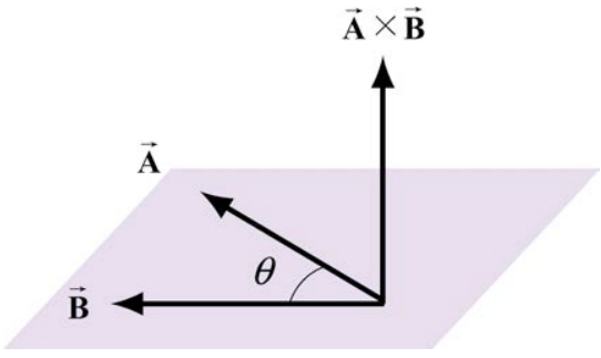
La dirección del producto vectorial se define de la siguiente manera. Los vectores\(\overrightarrow{\mathbf{A}}\) y\(\overrightarrow{\mathbf{B}}\) forman un plano. Considera la dirección perpendicular a este plano. Hay dos posibilidades: elegiremos una de estas dos (la que se muestra en la Figura 17.2) para la dirección del producto vectorial\(\overrightarrow{\mathbf{A}} \times \overrightarrow{\mathbf{B}}\) utilizando una convención que comúnmente se llama la “regla de la derecha”.

Regla de la mano derecha para la dirección del producto vectorial

El primer paso es volver a dibujar los vectores\(\overrightarrow{\mathbf{A}} \text { and } \overrightarrow{\mathbf{B}}\) para que las colas se toquen. Después dibuja un arco partiendo del vector\(\overrightarrow{\mathbf{A}}\) y terminando sobre el vector\(\overrightarrow{\mathbf{B}}\). Enroscar los dedos derechos de la misma manera que el arco. Su pulgar derecho apunta en la dirección del producto vectorial\(\overrightarrow{\mathbf{A}} \times \overrightarrow{\mathbf{B}}\) (Figura 17.3).

Figura 17.3 Regla de la mano derecha.

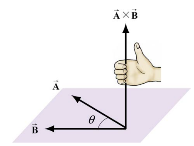
Debe recordar que la dirección del producto vectorial\(\overrightarrow{\mathbf{A}} \times \overrightarrow{\mathbf{B}}\) es perpendicular al plano formado por\(\overrightarrow{\mathbf{A}} \text { and } \overrightarrow{\mathbf{B}}\). Podemos dar una interpretación geométrica a la magnitud del producto vectorial escribiendo la magnitud como

\[|\overrightarrow{\mathbf{A}} \times \overrightarrow{\mathbf{B}}|=|\overrightarrow{\mathbf{A}}|(|\overrightarrow{\mathbf{B}}| \sin \theta) \nonumber \]

Los vectores\(\overrightarrow{\mathbf{A}} \text { and } \overrightarrow{\mathbf{B}}\) forman un paralelogramo. El área del paralelogramo es igual a la altura por la base, que es la magnitud del producto vectorial. En la Figura 17.4 se ilustran dos representaciones diferentes de la altura y base de un paralelogramo. Como se representa en la Figura 17.4a, el término\(|\overrightarrow{\mathbf{B}}| \sin \theta\) es la proyección del vector\(\overrightarrow{\mathbf{B}}\) en la dirección perpendicular al vector También\(\overrightarrow{\mathbf{B}}\) podríamos escribir la magnitud del producto vectorial como

\[|\overrightarrow{\mathbf{A}} \times \overrightarrow{\mathbf{B}}|=(|\overrightarrow{\mathbf{A}}| \sin \theta)|\overrightarrow{\mathbf{B}}| \nonumber \]

El término\(|\overrightarrow{\mathbf{A}}| \sin \theta\) es la proyección del vector\(\overrightarrow{\mathbf{A}}\) en la dirección perpendicular al vector\(\overrightarrow{\mathbf{B}}\) como se muestra en la Figura 17.4 (b). El producto vectorial de dos vectores que son paralelos (o antiparalelos) entre sí es cero porque el ángulo entre los vectores es 0 (o\(\pi\)) y\(\sin (0)=0\) (o\(\sin (\pi)=0\)). Geométricamente, dos vectores paralelos no tienen un componente único perpendicular a su dirección común.

Figura 17.4 Proyección de (a)\(\overrightarrow{\mathbf{B}}\) perpendicular a\(\overrightarrow{\mathbf{A}}\), (b) de\(\overrightarrow{\mathbf{A}}\) perpendicular a\(\overrightarrow{\mathbf{B}}\)

Propiedades del Producto Vector

(1) El producto vectorial es anticonmutativo porque cambiar el orden de los vectores cambia la dirección del producto vectorial por la regla de la derecha:

\[\overrightarrow{\mathbf{A}} \times \overrightarrow{\mathbf{B}}=-\overrightarrow{\mathbf{B}} \times \overrightarrow{\mathbf{A}} \nonumber \]

(2) El producto vectorial entre un vector\(c \overrightarrow{\mathbf{A}}\) donde\(c\) es un escalar y un vector\(\overrightarrow{\mathbf{B}}\) es

\[c \overrightarrow{\mathbf{A}} \times \overrightarrow{\mathbf{B}}=c(\overrightarrow{\mathbf{A}} \times \overrightarrow{\mathbf{B}}) \nonumber \]

Del mismo modo,

\[\overrightarrow{\mathbf{A}} \times c \overrightarrow{\mathbf{B}}=c(\overrightarrow{\mathbf{A}} \times \overrightarrow{\mathbf{B}}) \nonumber \]

(3) El producto vectorial entre la suma de dos vectores\(\overrightarrow{\mathbf{A}} \text { and } \overrightarrow{\mathbf{B}}\) con un vector\(\overrightarrow{\mathbf{C}}\) es

\[(\overrightarrow{\mathbf{A}}+\overrightarrow{\mathbf{B}}) \times \overrightarrow{\mathbf{C}}=\overrightarrow{\mathbf{A}} \times \overrightarrow{\mathbf{C}}+\overrightarrow{\mathbf{B}} \times \overrightarrow{\mathbf{C}} \nonumber \]

Del mismo modo,

\[\overrightarrow{\mathbf{A}} \times(\overrightarrow{\mathbf{B}}+\overrightarrow{\mathbf{C}})=\overrightarrow{\mathbf{A}} \times \overrightarrow{\mathbf{B}}+\overrightarrow{\mathbf{A}} \times \overrightarrow{\mathbf{C}} \nonumber \]

Descomposición vectorial y el producto vectorial: Coordenadas Cartesianas

Primero calculamos que la magnitud del producto vectorial de los vectores unitarios\(\hat{\mathbf{i}}\) y\(\hat{\mathbf{j}}\):

\[|\hat{\mathbf{i}} \times \hat{\mathbf{j}}|=|\hat{\mathbf{i}} \| \hat{\mathbf{j}}| \sin (\pi / 2)=1 \nonumber \]

porque los vectores unitarios tienen magnitud\(|\hat{\mathbf{i}}|=|\hat{\mathbf{j}}|=1\) y\(\sin (\pi / 2)=1\). Por la regla de la mano derecha, la dirección de\(\hat{\mathbf{i}} \times \hat{\mathbf{j}}\) está en el\(+\hat{\mathbf{k}}\) como se muestra en la Figura 17.5. Así\(\hat{\mathbf{i}} \times \hat{\mathbf{j}}=\hat{\mathbf{k}}\).

Figura 17.5 Producto vectorial de\(\hat{\mathbf{i}} \times \hat{\mathbf{j}}\)

Observamos que la misma regla se aplica para los vectores unitarios en las direcciones y y z,

\[\hat{\mathbf{j}} \times \hat{\mathbf{k}}=\hat{\mathbf{i}}, \quad \hat{\mathbf{k}} \times \hat{\mathbf{i}}=\hat{\mathbf{j}} \nonumber \]

Por la propiedad anticonmutativa (1) del producto vector,

\[\hat{\mathbf{j}} \times \hat{\mathbf{i}}=-\hat{\mathbf{k}}, \quad \hat{\mathbf{i}} \times \hat{\mathbf{k}}=-\hat{\mathbf{j}} \nonumber \]

El producto vectorial del vector unitario\(\hat{\mathbf{i}}\) consigo mismo es cero porque los dos vectores unitarios son paralelos entre sí\((\sin (0)=0)\),

\[|\hat{\mathbf{i}} \times \hat{\mathbf{i}}|=|\hat{\mathbf{i}}||\hat{\mathbf{i}}| \sin (0)=0 \nonumber \]

El producto vectorial del vector unitario\(\hat{\mathbf{j}}\) consigo mismo y el vector unitario\(\hat{\mathbf{k}}\) consigo mismo también son cero por la misma razón,

\[|\hat{\mathbf{j}} \times \hat{\mathbf{j}}|=0, \quad|\hat{\mathbf{k}} \times \hat{\mathbf{k}}|=0 \nonumber \]

Con estas propiedades en mente, ahora podemos desarrollar una expresión algebraica para el producto vector en términos de componentes. Escojamos un sistema de coordenadas cartesianas con el vector\(\overrightarrow{\mathbf{B}}\) apuntando a lo largo del eje x positivo con componente x positivo\(B_{x}\). Entonces los vectores\(\overrightarrow{\mathbf{A}} \text { and } \overrightarrow{\mathbf{B}}\) se pueden escribir como

\[\overrightarrow{\mathbf{A}}=A_{x} \hat{\mathbf{i}}+A_{y} \hat{\mathbf{j}}+A_{z} \hat{\mathbf{k}} \nonumber \]

\[\overrightarrow{\mathbf{B}}=B_{x} \hat{\mathbf{i}} \nonumber \]

respectivamente. El producto del vector en los componentes del vector es

\[\overrightarrow{\mathbf{A}} \times \overrightarrow{\mathbf{B}}=\left(A_{x} \hat{\mathbf{i}}+A_{y} \hat{\mathbf{j}}+A_{z} \hat{\mathbf{k}}\right) \times B_{x} \hat{\mathbf{i}} \nonumber \]

Esto se convierte,

\ [\ begin {aligned}
\ overrightarrow {\ mathbf {A}}\ times\ overrightarrow {\ mathbf {B}} &=\ left (A_ {x}\ hat {\ mathbf {i}}\ times B_ {x}\ hat {\ mathbf {i}}\ right) +\ left (A_ {y}\ hat {\ mathbf {j}\ veces B_ {x}\ sombrero {\ mathbf {i}}\ derecha) +\ izquierda (A_ {z}\ sombrero {\ mathbf {k}}\ veces B_ {x}\ sombrero {\ mathbf {i}}\ derecha)\\
&=A_ {x} B_ {x} (\ hat {\ mathbf {i}}\ times\ hat {\ mathbf {i}}) +A_ {y} B_ {x} (\ hat {\ mathbf {j}}\ times\ hat {\ mathbf {i}}) +A_ {z} B_ {x} (\ hat {\ mathbf {k}}\ tiempos\ hat {\ mathbf {i}})\\
&=-A_ {y} B_ {x}\ sombrero {\ mathbf {k}} +A_ {z} B_ {x}\ sombrero {\ mathbf {j}}
\ end {alineado}\ nonumber\]

La expresión del componente del vector para el producto vector generaliza fácilmente para vectores arbitrarios

\[\overrightarrow{\mathbf{A}}=A_{x} \hat{\mathbf{i}}+A_{y} \hat{\mathbf{j}}+A_{z} \hat{\mathbf{k}} \nonumber \]

\[\overrightarrow{\mathbf{B}}=B_{x} \hat{\mathbf{i}}+B_{y} \hat{\mathbf{j}}+B_{z} \hat{\mathbf{k}} \nonumber \]

para rendir

\[\overrightarrow{\mathbf{A}} \times \overrightarrow{\mathbf{B}}=\left(A_{y} B_{z}-A_{z} B_{y}\right) \hat{\mathbf{i}}+\left(A_{z} B_{x}-A_{x} B_{z}\right) \hat{\mathbf{j}}+\left(A_{x} B_{y}-A_{y} B_{x}\right) \hat{\mathbf{k}} \nonumber \]

Descomposición vectorial y el producto vectorial: Coordenadas Cilíndricas

Recordemos el sistema de coordenadas cilíndricas, que mostramos en la Figura 17.6. Hemos elegido dos direcciones, radial y tangencial en el plano, y una dirección perpendicular al plano.

Figura 17.6 Coordenadas cilíndricas

Los vectores unitarios están en ángulo recto entre sí y, por lo tanto, usando la regla de la derecha, el producto vectorial de los vectores unitarios viene dado por las relaciones

\[\hat{\mathbf{r}} \times \hat{\boldsymbol{\theta}}=\hat{\mathbf{k}} \nonumber \]

\[\hat{\boldsymbol{\theta}} \times \hat{\mathbf{k}}=\hat{\mathbf{r}} \nonumber \]

\[\hat{\mathbf{k}} \times \hat{\mathbf{r}}=\hat{\boldsymbol{\theta}} \nonumber \]

Porque el producto vectorial satisface también\(\overrightarrow{\mathbf{A}} \times \overrightarrow{\mathbf{B}}=-\overrightarrow{\mathbf{B}} \times \overrightarrow{\mathbf{A}}\) tenemos eso

\[\hat{\boldsymbol{\theta}} \times \hat{\mathbf{r}}=-\hat{\mathbf{k}} \nonumber \]

\[\hat{\mathbf{k}} \times \hat{\boldsymbol{\theta}}=-\hat{\mathbf{r}} \nonumber \]

\[\hat{\mathbf{r}} \times \hat{\mathbf{k}}=-\hat{\boldsymbol{\theta}} \nonumber \]

Finalmente

\[\hat{\mathbf{r}} \times \hat{\mathbf{r}}=\hat{\boldsymbol{\theta}} \times \hat{\boldsymbol{\theta}}=\hat{\mathbf{k}} \times \hat{\mathbf{k}}=\overrightarrow{\mathbf{0}} \nonumber \]

Ejemplo 17.1 Productos vectoriales

Dados dos vectores,\(\overrightarrow{\mathbf{A}}=2 \hat{\mathbf{i}}+-3 \hat{\mathbf{j}}+7 \hat{\mathbf{k}}\) y\(\overrightarrow{\mathbf{B}}=5 \hat{\mathbf{i}}+\hat{\mathbf{j}}+2 \hat{\mathbf{k}}\), encontrar\(\overrightarrow{\mathbf{A}} \times \overrightarrow{\mathbf{B}}\).

Solución:

\ [\ begin {alineado}
\ overrightarrow {\ mathbf {A}}\ times\ overrightarrow {\ mathbf {B}} &=\ left (A_ {y} B_ {z} -A_ {z} B_ {y}\ derecha)\ hat {\ mathbf {i}} +\ left (A_ {z} B_ {x} -A_ {x} B_ {z}\ derecha)\ sombrero {\ mathbf {j}} +\ izquierda (A_ {x} B_ {y} -A_ {y} B_ {x}\ derecha)\ sombrero {\ mathbf {k}}\\
& =( (-3) (2) - (7) (1))\ sombrero {\ mathbf {i}} + ((7) (5) - (2) (2))\ hat {\ mathbf {j}} + ((2) (1) - (-3) (5))\ hat {\ mathbf {k}}\\
&=-13\ hat {\ mathbf {i}} +31\ hat {\ mathbf {j}} +17\ hat {\ mathbf {k}}
\ final {alineado}\ nonumber\]

Ejemplo 17.2 Ley de los senos

Para el triángulo mostrado en la Figura 17.7a, probar la ley de los senos,\(|\overrightarrow{\mathbf{A}}| / \sin \alpha=|\overrightarrow{\mathbf{B}}| / \sin \beta=|\overrightarrow{\mathbf{C}}| / \sin \gamma\), utilizando el producto vectorial.

Figura 17.7 (b) Análisis vectorial

Solución: Considere el área de un triángulo formado por tres vectores\(\overrightarrow{\mathbf{A}}, \overrightarrow{\mathbf{B}}\), y\(\overrightarrow{\mathbf{C}}\), dónde\(\overrightarrow{\mathbf{A}}+\overrightarrow{\mathbf{B}}+\overrightarrow{\mathbf{C}}=0\) (Figura 17.7b). Porque\(\overrightarrow{\mathbf{A}}+\overrightarrow{\mathbf{B}}+\overrightarrow{\mathbf{C}}=0\), tenemos eso\(0=\overrightarrow{\mathbf{A}} \times(\overrightarrow{\mathbf{A}}+\overrightarrow{\mathbf{B}}+\overrightarrow{\mathbf{C}})=\overrightarrow{\mathbf{A}} \times \overrightarrow{\mathbf{B}}+\overrightarrow{\mathbf{A}} \times \overrightarrow{\mathbf{C}}\). Así\(\overrightarrow{\mathbf{A}} \times \overrightarrow{\mathbf{B}}=-\overrightarrow{\mathbf{A}} \times \overrightarrow{\mathbf{C}}\) o\(|\overrightarrow{\mathbf{A}} \times \overrightarrow{\mathbf{B}}|=|\overrightarrow{\mathbf{A}} \times \overrightarrow{\mathbf{C}}|\). De la Figura 17.7b vemos que\(|\overrightarrow{\mathbf{A}} \times \overrightarrow{\mathbf{B}}|=|\overrightarrow{\mathbf{A}}||\overrightarrow{\mathbf{B}}| \sin \gamma\) y\(|\overrightarrow{\mathbf{A}} \times \overrightarrow{\mathbf{C}}|=|\overrightarrow{\mathbf{A}}||\overrightarrow{\mathbf{C}}| \sin \beta\). Por lo tanto\(|\overrightarrow{\mathbf{A}}||\overrightarrow{\mathbf{B}}| \sin \gamma=|\overrightarrow{\mathbf{A}}||\overrightarrow{\mathbf{C}}| \sin \beta\), y por lo tanto\(|\overrightarrow{\mathbf{B}}| / \sin \beta=|\overrightarrow{\mathbf{C}}| / \sin \gamma\). Un argumento similar muestra que\(|\overrightarrow{\mathbf{B}}| / \sin \beta=|\overrightarrow{\mathbf{A}}| / \sin \alpha\) probar la ley de los senos.

Ejemplo 17.3 Unidad Normal

Encuentra un vector unitario perpendicular a\(\overrightarrow{\mathbf{A}}=\hat{\mathbf{i}}+\hat{\mathbf{j}}-\hat{\mathbf{k}}\) y\(\overrightarrow{\mathbf{B}}=-2 \hat{\mathbf{i}}-\hat{\mathbf{j}}+3 \hat{\mathbf{k}}\).

Solución: El producto vectorial\(\overrightarrow{\mathbf{A}} \times \overrightarrow{\mathbf{B}}\) es perpendicular a ambos\(\overrightarrow{\mathbf{A}} \text { and } \overrightarrow{\mathbf{B}}\). Por lo tanto, los vectores unitarios\(\hat{\mathbf{n}}=\pm \overrightarrow{\mathbf{A}} \times \overrightarrow{\mathbf{B}} /|\overrightarrow{\mathbf{A}} \times \overrightarrow{\mathbf{B}}|\) son perpendiculares a ambos\(\overrightarrow{\mathbf{A}} \text { and } \overrightarrow{\mathbf{B}}\). Primero calculamos

\ [\ begin {alineado}
\ overrightarrow {\ mathbf {A}}\ times\ overrightarrow {\ mathbf {B}} &=\ left (A_ {y} B_ {z} -A_ {z} B_ {y}\ derecha)\ hat {\ mathbf {i}} +\ left (A_ {z} B_ {x} -A_ {x} B_ {z}\ derecha)\ sombrero {\ mathbf {j}} +\ izquierda (A_ {x} B_ {y} -A_ {y} B_ {x}\ derecha)\ sombrero {\ mathbf {k}}\\
& =( (1) (3) - (-1) (-1))\ sombrero {\ mathbf {i}} + ((-1) (2) - (1) (3))\ hat {\ mathbf {j}} + ((1) (-1) - (1) (2))\ hat {\ mathbf {k}}\\
&=2\ hat {\ mathbf {i}} -5\ sombrero {\ mathbf {j}} -3\ sombrero {\ mathbf {k}}
\ end {alineado}\ nonumber\]

Ahora calculamos la magnitud

\[|\overrightarrow{\mathbf{A}} \times \overrightarrow{\mathbf{B}}|=\left(2^{2}+5^{2}+3^{2}\right)^{1 / 2}=(38)^{1 / 2} \nonumber \]

Por lo tanto los vectores unitarios perpendiculares son

\[\hat{\mathbf{n}}=\pm \overrightarrow{\mathbf{A}} \times \overrightarrow{\mathbf{B}} /|\overrightarrow{\mathbf{A}} \times \overrightarrow{\mathbf{B}}|=\pm(2 \hat{\mathbf{i}}-5 \hat{\mathbf{j}}-3 \hat{\mathbf{k}}) /(38)^{1 / 2} \nonumber \]

Ejemplo 17.4 Volumen de Paralelepípedo

Mostrar que el volumen de un paralelepípedo con bordes formados por los vectores\(\overrightarrow{\mathbf{A}}, \overrightarrow{\mathbf{B}}, \text { and }\)\(\overrightarrow{\mathbf{C}}\) viene dado por\(\overrightarrow{\mathbf{A}} \cdot(\overrightarrow{\mathbf{B}} \times \overrightarrow{\mathbf{C}})\).

Solución: El volumen de un paralelepípedo viene dado por el área de la base veces la altura. Si la base está formada por los vectores\(\overrightarrow{\mathbf{B}} \text { and } \overrightarrow{\mathbf{C}}\), entonces el área de la base viene dada por la magnitud de\(\overrightarrow{\mathbf{B}} \times \overrightarrow{\mathbf{C}}\). El vector\(\overrightarrow{\mathbf{B}} \times \overrightarrow{\mathbf{C}}=|\overrightarrow{\mathbf{B}} \times \overrightarrow{\mathbf{C}}| \hat{\mathbf{n}}\) donde\(\hat{\mathbf{n}}\) es un vector unitario perpendicular a la base (Figura 17.8).

Figura 17.8 Ejemplo 17.4

La proyección del vector\(\overrightarrow{\mathbf{A}}\) a lo largo de la dirección\(\hat{\mathbf{n}}\) da la altura del paralelepípedo. Esta proyección se da tomando el producto punto de\(\overrightarrow{\mathbf{A}}\) con un vector unitario y es igual a\(\overrightarrow{\mathbf{A}} \cdot \hat{\mathbf{n}}=\text { height }\). Por lo tanto

\[\overrightarrow{\mathbf{A}} \cdot(\overrightarrow{\mathbf{B}} \times \overrightarrow{\mathbf{C}})=\overrightarrow{\mathbf{A}} \cdot(|\overrightarrow{\mathbf{B}} \times \overrightarrow{\mathbf{C}}|) \hat{\mathbf{n}}=(|\overrightarrow{\mathbf{B}} \times \overrightarrow{\mathbf{C}}|) \overrightarrow{\mathbf{A}} \cdot \hat{\mathbf{n}}=(\text { area })(\text { height })=(\text { volume }) \nonumber \]

Ejemplo 17.5 Descomposición vectorial

Dejar\(\overrightarrow{\mathbf{A}}\) ser un vector arbitrario y dejar\(\hat{\mathbf{n}}\) ser un vector unitario en alguna dirección fija. Demostrar que\(\overrightarrow{\mathbf{A}}=(\overrightarrow{\mathbf{A}} \cdot \hat{\mathbf{n}}) \hat{\mathbf{n}}+(\hat{\mathbf{n}} \times \overrightarrow{\mathbf{A}}) \times \hat{\mathbf{n}}\)

Solución: Dejar\(\overrightarrow{\mathbf{A}}=A_{\|} \hat{\mathbf{n}}+A_{\perp} \hat{\mathbf{e}}\) donde\(A_{\|}\) está el componente\(\overrightarrow{\mathbf{A}}\) en la dirección de\(\hat{\mathbf{n}}, \hat{\mathbf{e}}\) es la dirección de la proyección de\(\overrightarrow{\mathbf{A}}\) en un plano perpendicular a\(\hat{\mathbf{n}}\), y\(A_{\perp}\) es el componente de\(\overrightarrow{\mathbf{A}}\) en la dirección de\(\hat{\mathbf{e}}\). Porque\(\hat{\mathbf{e}} \cdot \hat{\mathbf{n}}=0\), tenemos eso\(\overrightarrow{\mathbf{A}} \cdot \hat{\mathbf{n}}=A_{\|}\). Tenga en cuenta que

\[\hat{\mathbf{n}} \times \overrightarrow{\mathbf{A}}=\hat{\mathbf{n}} \times\left(A \hat{\mathbf{n}}+A_{\perp} \hat{\mathbf{e}}\right)=\hat{\mathbf{n}} \times A_{\perp} \hat{\mathbf{e}}=A_{\perp}(\hat{\mathbf{n}} \times \hat{\mathbf{e}}) \nonumber \]

El vector unitario\(\hat{\mathbf{n}} \times \hat{\mathbf{e}}\) se encuentra en el plano perpendicular a\(\hat{\mathbf{n}}\) y también es perpendicular al\(\hat{\mathbf{e}}\). Por lo tanto, también\((\hat{\mathbf{n}} \times \hat{\mathbf{e}}) \times \hat{\mathbf{n}}\) es un vector unitario que es paralelo a\(\hat{\mathbf{e}}\) (por la regla de la mano derecha. Entonces\((\hat{\mathbf{n}} \times \overrightarrow{\mathbf{A}}) \times \hat{\mathbf{n}}=A_{\perp} \hat{\mathbf{e}}\). Así

\[\overrightarrow{\mathbf{A}}=A_{\|} \hat{\mathbf{n}}+A_{\perp} \hat{\mathbf{e}}=(\overrightarrow{\mathbf{A}} \cdot \hat{\mathbf{n}}) \hat{\mathbf{n}}+(\hat{\mathbf{n}} \times \overrightarrow{\mathbf{A}}) \times \hat{\mathbf{n}} \nonumber \]