22.2: Giroscopio

Un giroscopio de masa de juguete\(m\) consiste en un volante giratorio montado en un bastidor de suspensión que permite que el eje del volante apunte en cualquier dirección. Un extremo del eje está soportado sobre una\(a\) distancia\(d\) de pilón desde el centro de masa del giroscopio.

Figura 22.2: un giroscopio de juguete

Elija coordenadas polares para que el eje del volante del giroscopio quede alineado a lo largo del eje r y el eje vertical sea el eje z (la Figura 22.2 muestra una representación esquemática del giroscopio).

Figura 22.3 Rotaciones angulares

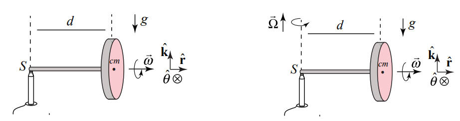
El volante gira alrededor de su eje con una velocidad angular de giro,

\[\overrightarrow{\boldsymbol{\omega}}_{s}=\omega_{s} \hat{\mathbf{r}} \nonumber \]

donde\(\omega_{s}\) está el componente radial y\(\omega_{s}>0\) para el caso ilustrado en la Figura 22.2.

Cuando soltamos el giroscopio sufre un movimiento muy sorprendente. En lugar de caer hacia abajo, el centro de masa gira alrededor de un eje vertical que pasa por el punto\(S\) de contacto del eje con el pilón con una velocidad angular precessional

\[\overrightarrow{\boldsymbol{\Omega}}=\Omega_{z} \hat{\mathbf{k}}=\frac{d \theta}{d t} \hat{\mathbf{k}} \nonumber \]

donde\(\Omega_{z}=d \theta / d t\) está el componente z y\(\Omega_{z}>0\) para el caso ilustrado en la Figura 22.3. Por lo tanto, la velocidad angular del volante es la suma de estas dos contribuciones

\[\overrightarrow{\boldsymbol{\omega}}=\overrightarrow{\boldsymbol{\omega}}_{s}+\overrightarrow{\boldsymbol{\Omega}}=\omega_{s} \hat{\mathbf{r}}+\Omega_{z} \hat{\mathbf{k}} \nonumber \]

Estudiaremos el caso especial donde la magnitud del componente de precesión\(\left|\Omega_{z}\right|\) de la velocidad angular es mucho menor que la magnitud de la componente de giro\(\left|\omega_{s}\right|\) de la velocidad angular de giro\(\left|\Omega_{z}\right|<<\mid \omega_{s}\), de manera que la magnitud de la velocidad angular sea\(|\vec{\omega}| \simeq\left|\omega_{\mathrm{s}}\right| \text { and } \Omega_{z} \text { and } \omega_{s}\) casi constante. Estos supuestos se denominan colectivamente la aproximación giroscópica.

El diagrama de fuerza para el giroscopio se muestra en la Figura 22.4. La fuerza gravitacional actúa en el centro de la masa y se dirige hacia abajo,\(\overrightarrow{\mathbf{F}}^{g}=-m g \hat{\mathbf{k}}\). También hay una fuerza de contacto,\(\overrightarrow{\mathbf{F}}^{c}\) entre el extremo del eje y el pilón. Puede parecer que la fuerza de contacto,\(\overrightarrow{\mathbf{F}}^{c}\) tiene sólo una componente ascendente\(\overrightarrow{\mathbf{F}}^{v}=F_{z} \hat{\mathbf{k}}\), pero como pronto veremos también debe haber una componente radial hacia adentro a la fuerza de contacto,\(\overrightarrow{\mathbf{F}}^{r}=F_{r} \hat{\mathbf{r}}, \text { with } F_{r}<0\) porque el centro de masa experimenta un movimiento circular.

Figura 22.4 Diagrama de fuerza y par para el giroscopio

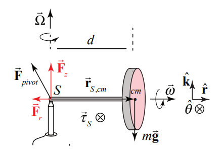
La razón por la que el giroscopio no se cae es que la componente vertical de la fuerza de contacto equilibra exactamente la fuerza gravitacional

\[F_{z}-m g=0 \nonumber \]

¿Qué pasa con el par sobre el punto de contacto\(S\)? La fuerza de contacto actúa\(S\) por lo que no contribuye al par alrededor\(S\); solo la fuerza gravitacional contribuye al par alrededor\(S\) (Figura 22.5b). La dirección del par alrededor\(S\) viene dada por

\[\vec{\tau}_{S}=\overrightarrow{\mathbf{r}}_{S, \mathrm{cm}} \times \overrightarrow{\mathbf{F}}_{\mathrm{gravity}}=d \hat{\mathbf{r}} \times m g(-\hat{\mathbf{k}})=d m g \hat{\boldsymbol{\theta}} \nonumber \]

y está en la\(\hat{\boldsymbol{\theta}}\) dirección positiva. Sin embargo sabemos que si hay un par distinto de cero alrededor\(S\), entonces el momento angular alrededor\(S\) debe cambiar en el tiempo, según

\[\vec{\tau}_{S}=\frac{d \overrightarrow{\mathrm{L}}_{S}}{d t} \nonumber \]

El momento angular alrededor del punto\(S\) del giroscopio viene dado por

\[\overrightarrow{\mathbf{L}}_{S}=\overrightarrow{\mathbf{L}}_{S}^{\text {otbital }}+\overrightarrow{\mathbf{L}}_{\mathrm{cm}}^{\text {spin }} \nonumber \]

El momento angular orbital alrededor del punto\(S\) es

\[\overrightarrow{\mathbf{L}}_{S}^{\text {otbial }}=\overrightarrow{\mathbf{r}}_{S, c m} \times m \overrightarrow{\mathbf{v}}_{c m}=d \hat{\mathbf{r}} \times m d \Omega_{z} \hat{\boldsymbol{\theta}}=m d^{2} \Omega_{z} \hat{\mathbf{k}} \nonumber \]

La magnitud del momento angular orbital\(S\) es casi constante y la dirección no cambia. Por lo tanto

\[\frac{d}{d t} \overrightarrow{\mathbf{L}}_{S}^{\text {obital }}=\overrightarrow{\mathbf{0}} \nonumber \]

El momento angular de giro incluye dos términos. Recordemos que el volante se somete a dos rotaciones separadas alrededor de diferentes ejes. Está girando alrededor del eje del volante con velocidad angular de giro\(\overrightarrow{\boldsymbol{\omega}}_{s}\). A medida que el volante precede alrededor del punto de pivote, el volante gira alrededor del eje z con velocidad angular de precesión\(\overrightarrow{\mathbf{\Omega}}\) (Figura 22.5). Por lo tanto, el momento angular de giro viene dado por

\[\overrightarrow{\mathbf{L}}_{\mathrm{cm}}^{\operatorname{spin}}=I_{r} \omega_{s} \hat{\mathbf{r}}+I_{z} \Omega_{z} \hat{\mathbf{k}} \nonumber \]

donde\(I_{r}\) es el momento de inercia con respecto al eje del volante y\(I_{z}\) es el momento de inercia con respecto al eje z. Si asumimos que el eje es sin masa y el volante es uniforme con radio R, entonces\(I_{r}=(1 / 2) m R^{2}\). Por el teorema del eje perpendicular de\(I_{r}=I_{z}+I_{y}=2 I_{z}\) ahí\(I_{z}=(1 / 4) m R^{2}\).

Figura 22.5: Rotaciones alrededor del centro de masa del volante Figura 22.6 Momento angular de giro.

Recordemos que la aproximación giroscópica se mantiene cuando lo\(\left|\Omega_{z}\right|<<\left|\omega_{s}\right|\) que implica eso\(I_{z} \Omega_{z}<<I_{r} \omega_{s}\) y por lo tanto podemos ignorar la contribución al momento angular de giro desde la rotación alrededor del eje vertical, y así

\[\overrightarrow{\mathbf{L}}_{\mathrm{cm}}^{\operatorname{spin}} \simeq I_{\mathrm{cm}} \omega_{s} \hat{\mathbf{r}} \nonumber \]

(La contribución al momento angular de giro debido a la rotación alrededor del eje z,\(I_{z} \Omega_{z} \hat{\mathbf{k}}\) es casi constante tanto en magnitud como en dirección por lo que no cambia en el tiempo,\(d\left(I_{z} \Omega_{z} \hat{\mathbf{k}}\right) / d t \simeq \overrightarrow{\mathbf{0}}\). Por lo tanto, el momento angular\(S\) es aproximadamente

\[\overrightarrow{\mathbf{L}}_{S} \simeq \overrightarrow{\mathbf{L}}_{\mathrm{cm}}^{\mathrm{spin}}=I_{\mathrm{cm}} \omega_{s} \hat{\mathbf{r}} \nonumber \]

Nuestra expectativa inicial de que el giroscopio caiga hacia abajo debido al par que la fuerza gravitacional ejerce sobre el punto de contacto\(S\) conduce a una violación de la ley de par. Si el centro de masa comenzara a caer entonces el cambio en el momento angular del giro,\(\Delta \overrightarrow{\mathbf{L}}_{\mathrm{cm}}^{\operatorname{spin}}\) apuntaría en la dirección z negativa y eso contradiría el aspecto vectorial de la Ecuación (22.2.6). En lugar de caer hacia abajo, el momento angular alrededor del centro de masa,\(\overrightarrow{\mathbf{L}}_{\mathrm{cm}}^{\mathrm{spin}}\) debe cambiar de dirección de tal manera que la dirección de\(\Delta \overrightarrow{\mathbf{L}}_{\mathrm{cm}}^{\text {spin }}\) esté en la misma dirección que el par sobre\(S\) (Ecuación (22.2.5)), la\(\hat{\boldsymbol{\theta}}\) dirección positiva.

Recordemos que en nuestro estudio del movimiento circular, ya nos hemos encontrado con varios ejemplos en los que cambia la dirección de un vector de magnitud constante. Consideramos un objeto puntual de masa m moviéndose en un círculo de radio r. Cuando elegimos un sistema de coordenadas con un origen en el centro del círculo, el vector de posición\(\overrightarrow{\mathbf{r}}\) se dirige radialmente hacia afuera. A medida que la masa se mueve en círculo, el vector de posición tiene una magnitud constante pero cambia de dirección. El vector de velocidad viene dado por

\[\overrightarrow{\mathbf{v}}=\frac{d \overrightarrow{\mathbf{r}}}{d t}=\frac{d}{d t}(r \hat{\mathbf{r}})=r \frac{d \theta}{d t} \hat{\boldsymbol{\theta}}=r \omega_{z} \hat{\boldsymbol{\theta}} \nonumber \]

y tiene dirección que es perpendicular al vector de posición (tangente al círculo), (Figura 22.7a)).

Figura 22.7 (a) Vector de posición y velocidad de rotación; (b) vector de velocidad y aceleración para un movimiento circular uniforme

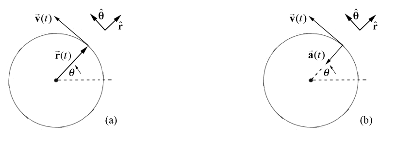
Para un movimiento circular uniforme, la magnitud de la velocidad es constante pero la dirección cambia constantemente y encontramos que la aceleración viene dada por (Figura 22.7b)

\[\overrightarrow{\mathbf{a}}=\frac{d \overrightarrow{\mathbf{v}}}{d t}=\frac{d}{d t}\left(v_{\theta} \hat{\boldsymbol{\theta}}\right)=v_{\theta} \frac{d \theta}{d t}(-\hat{\mathbf{r}})=r \omega_{z} \omega_{z}(-\hat{\mathbf{r}})=-r \omega_{z}^{2} \hat{\mathbf{r}} \nonumber \]

Tenga en cuenta que utilizamos los hechos que

\ [\ begin {array} {l}
\ frac {d\ hat {\ mathbf {r}}} {d t} =\ frac {d\ theta} {d t}\ hat {\ boldsymbol {\ theta}}
\\ frac {d\ theta} {d\ theta}} {d t} =-\ frac {d\ theta} d t}\ hat {\ mathbf {r}}
\ end {array}\ nonumber\]

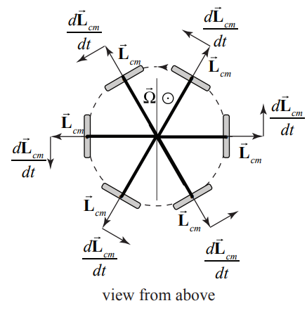
en Ecuaciones (22.2.13) y (22.2.14). Podemos aplicar el mismo razonamiento a cómo cambia el ángulo de giro en el tiempo (Figura 22.8).

La derivada de tiempo del momento angular de giro viene dada por

\[\frac{d \overrightarrow{\mathbf{L}}_{S}}{d t}=\frac{d \overrightarrow{\mathbf{L}}_{\mathrm{cm}, \omega_{s}}^{\operatorname{spin}}}{d t}=\left|\overrightarrow{\mathbf{L}}_{\mathrm{cm}, \omega_{s}}^{\sin }\right| \frac{d \theta}{d t} \hat{\boldsymbol{\theta}}=\left|\overrightarrow{\mathbf{L}}_{\mathrm{cm}, \omega_{s}}^{\sin }\right| \Omega_{z} \hat{\boldsymbol{\theta}}=I_{r} \omega_{s} \Omega_{z} \hat{\boldsymbol{\theta}} \nonumber \]

donde\(\Omega_{z}=d \theta / d t\) está el componente z y\(\Omega_{z}>0\). El centro de masa del volante gira alrededor de un eje vertical que pasa por el punto\(S\) de contacto del eje con el pilón con una velocidad angular precessional.

\[\overrightarrow{\mathbf{Q}}=\Omega_{z} \hat{\mathbf{k}}=\frac{d \theta}{d t} \hat{\mathbf{k}} \nonumber \]

Sustituir las ecuaciones (22.2.16) y (22.2.5) en la ecuación (22.2.6) rindiendo

\[d m g \hat{\boldsymbol{\theta}}=\left|\overrightarrow{\mathbf{L}}_{\mathrm{cm}}^{\sin }\right| \Omega_{z} \hat{\boldsymbol{\theta}} \nonumber \]

Resolviendo la ecuación (22.2.18) para el componente z de la velocidad angular precessional de los rendimientos del giroscopio

\[\Omega_{z}=\frac{d m g}{\left|\overrightarrow{\mathbf{L}}_{\mathrm{cm}}^{\mathrm{spin}}\right|}=\frac{d m g}{I_{\mathrm{cm}} \omega_{\mathrm{s}}} \nonumber \]

Figura 22.8 Cambio de dirección de tiempo del momento angular de giro