
15.2: Descompresión adiabática
- Page ID
- 127795

\( \newcommand{\vecs}[1]{\overset { \scriptstyle \rightharpoonup} {\mathbf{#1}} } \)
\( \newcommand{\vecd}[1]{\overset{-\!-\!\rightharpoonup}{\vphantom{a}\smash {#1}}} \)
\( \newcommand{\id}{\mathrm{id}}\) \( \newcommand{\Span}{\mathrm{span}}\)
( \newcommand{\kernel}{\mathrm{null}\,}\) \( \newcommand{\range}{\mathrm{range}\,}\)
\( \newcommand{\RealPart}{\mathrm{Re}}\) \( \newcommand{\ImaginaryPart}{\mathrm{Im}}\)
\( \newcommand{\Argument}{\mathrm{Arg}}\) \( \newcommand{\norm}[1]{\| #1 \|}\)
\( \newcommand{\inner}[2]{\langle #1, #2 \rangle}\)
\( \newcommand{\Span}{\mathrm{span}}\)
\( \newcommand{\id}{\mathrm{id}}\)
\( \newcommand{\Span}{\mathrm{span}}\)
\( \newcommand{\kernel}{\mathrm{null}\,}\)
\( \newcommand{\range}{\mathrm{range}\,}\)
\( \newcommand{\RealPart}{\mathrm{Re}}\)
\( \newcommand{\ImaginaryPart}{\mathrm{Im}}\)
\( \newcommand{\Argument}{\mathrm{Arg}}\)
\( \newcommand{\norm}[1]{\| #1 \|}\)
\( \newcommand{\inner}[2]{\langle #1, #2 \rangle}\)
\( \newcommand{\Span}{\mathrm{span}}\) \( \newcommand{\AA}{\unicode[.8,0]{x212B}}\)
\( \newcommand{\vectorA}[1]{\vec{#1}} % arrow\)
\( \newcommand{\vectorAt}[1]{\vec{\text{#1}}} % arrow\)
\( \newcommand{\vectorB}[1]{\overset { \scriptstyle \rightharpoonup} {\mathbf{#1}} } \)
\( \newcommand{\vectorC}[1]{\textbf{#1}} \)
\( \newcommand{\vectorD}[1]{\overrightarrow{#1}} \)
\( \newcommand{\vectorDt}[1]{\overrightarrow{\text{#1}}} \)
\( \newcommand{\vectE}[1]{\overset{-\!-\!\rightharpoonup}{\vphantom{a}\smash{\mathbf {#1}}}} \)
\( \newcommand{\vecs}[1]{\overset { \scriptstyle \rightharpoonup} {\mathbf{#1}} } \)
\( \newcommand{\vecd}[1]{\overset{-\!-\!\rightharpoonup}{\vphantom{a}\smash {#1}}} \)
Vamos a calcular una expresión para\((∂T/∂P)_S\). La expresión será positiva, ya que T y P aumentan juntos. Consideraremos la entropía como una función de temperatura y presión, y, con las variables
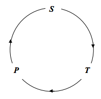
comenzaremos con la relación cíclica
\[\left(\frac{\partial S}{\partial T}\right)_{P}\left(\frac{\partial T}{\partial P}\right)_{S}\left(\frac{\partial P}{\partial S}\right)_{T}=-1. \label{15.2.1}\]
El término medio es el que queremos. Busquemos expresiones para la primera y tercera derivada parcial en términos de cosas que podamos medir.
En un proceso reversible\(dS = dQ/T\), y, en un proceso isobárico,\(dQ = C_PdT\). Por lo tanto
\[ \left(\frac{\partial S}{\partial T}\right)_{p}=\frac{C_{p}}{T}.\]
Además, tenemos una relación Maxwell (Ecuación 12.6.16). \(\left(\frac{\partial S}{\partial P}\right)_{T}=-\left(\frac{\partial V}{\partial T}\right)_{P}\). Así, la ecuación\ ref {15.2.1} se convierte en
\[\left(\frac{\partial T}{\partial P}\right)_{S}=\frac{T}{C_{P}}\left(\frac{\partial V}{\partial T}\right)_{P}. \label{15.2.2}\]
Consulta las dimensiones de este. Obsérvese también que C P puede ser total, específico o molar, siempre que V sea correspondientemente total, específico o molar. (T /P) S es, por supuesto, intensivo.
Si el gas es un gas ideal, la ecuación de estado es\(PV = RT\), de manera que
\[ \left(\frac{\partial V}{\partial T}\right)_{P}=\frac{R}{P}=\frac{V}{T}.\]
La ecuación\ ref {15.2.2} por lo tanto se convierte en
\[\left(\frac{\partial T}{\partial P}\right)_{S}=\frac{V}{C_{P}}.\]