3.9: Un modelo de circuito de señal pequeña

En la discusión del establecimiento del equilibrio entre un contacto y una molécula se introdujo un modelo de circuito generalizado donde cada potencial de nodo es el nivel Fermi, no el potencial electrostático como en un circuito eléctrico convencional.

Podemos extender el modelo a dos terminales, e incluso a tres dispositivos terminales. Debe enfatizarse, sin embargo, que el modelo sólo es válido para señales pequeñas. En particular, el modelo está restringido a pequeño\(V_{DS}\). Suponemos que la densidad de estados es constante y la modulación en\(V_{DS}\) debe ser menor que\(kT/q\) para que podamos ignorar las colas de la distribución de Fermi.

Consideremos la corriente inyectada por la fuente

\[ I_{S} = \frac{q}{\tau_{S}}(N_{S}-N) \nonumber \]

Esto se puede reescribir como

\[ I_{S} = \frac{q}{\tau_{S}}\int^{+\infty}_{-\infty} g(E-U)(f(E,\mu_{S})-f(E,E_{F}))dE \nonumber \]

Para pequeñas diferencias entre los potenciales de fuente y drenaje, y a T = 0K, obtenemos

\[ I_{S} = \frac{C_{Q}}{\tau_{S}}\frac{(\mu_{S}-E_{F})}{q} \nonumber \]

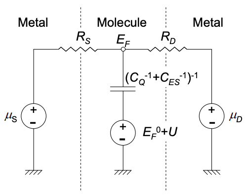
Así, cada interfaz contacto/molécula es óhmica en el límite de señal pequeña. Definición\(R_{S} = \tau_{S}/C_{Q}\), y\(R_{D} = \tau_{D}/C_{Q}\) .Podemos modelar el contacto/molécula/contacto como se muestra en la Figura 3.9.1.

Figura\(\PageIndex{1}\): Modelo de señal pequeña para dos circuitos terminales de metal/molécula/metal. Tenga en cuenta que el potencial U debe determinarse por separado (por ejemplo, mediante el uso de un circuito divisor capacitivo).