3.4: Forma de pendiente-interceptación de una línea

Comenzamos con la definición de la\(y\) -intercepción de una línea.

El\(y\)-intercept

El punto\((0,b)\) donde la gráfica de una línea cruza el\(y\) eje -se llama la\(y\) -intercepción de la línea.

Ahora vamos a generar la fórmula pendiente-intercepción para una línea que tiene\(y\) -intercept\((0,b)\) y\(\text {Slope} = m\) (ver Figura\(\PageIndex{1}\)). Déjese\((x,y)\) ser un punto arbitrario en la línea.

Figura\(\PageIndex{1}\): Línea con\(y\) -intercepción en\((0,b)\) y\(\text {Slope} = m\).

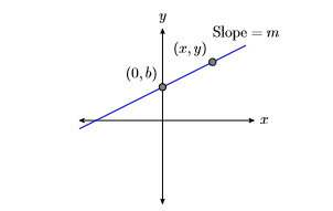
Comience con el hecho de que la pendiente de la línea es la velocidad a la que la variable dependiente está cambiando con respecto a la variable independiente.

\[\text {Slope} =\dfrac{\Delta y}{\Delta x} \qquad \color{Red} \text {Slope formula.} \nonumber \]

Sustituto\(m\) de la pendiente. Para determinar tanto el cambio en\(y\) como el cambio en\(x\), restar las coordenadas del punto\((0,b)\) del punto del punto\((x,y)\).

\[\begin{aligned} m&=\frac{y-b}{x-0} \quad \color {Red} \text { Substitute } m \text { for the Slope. } \Delta y =y-b \quad \color {Red} \text { and } \Delta x=x-0 .\\ m&=\frac{y-b}{x} \quad \color {Red}\text { Simplify. } \end{aligned} \nonumber \]

Borrar fracciones de la ecuación multiplicando ambos lados por el denominador común.

\[\begin{aligned} mx &= \left[\dfrac{y-b}{x}\right] x \quad \color {Red} \text { Multiply both sides by } x \\ mx &= y-b \quad \color {Red} \text { Cancel. } \end{aligned} \nonumber \]

Resolver para\(y\).

\[\begin{aligned} mx+b&= y-b+b \quad \color {Red} \text { Add } b \text { to both sides. } \\ mx+b&= y \quad \color {Red} \text { Simplify. } \end{aligned} \nonumber \]

Así, la ecuación de la línea es\(y = mx + b\).

La forma Slope-Intercept de una línea

La ecuación de la línea que tiene\(y\) intercepción\((0,b)\) y pendiente\(m\) es:\[y = mx + b \nonumber \] Debido a que esta forma de una línea depende de conocer la pendiente\(m\) y la intercepción\((0,b)\), esta forma se denomina la forma pendiente-intercepción de una línea.

Ejemplo\(\PageIndex{1}\)

Dibuje la gráfica de la línea que tiene ecuación\(y=\dfrac{3}{5} x+1\).

Solución

Compare la ecuación\(y=\dfrac{3}{5} x+1\) con la forma pendiente-intercepción\(y = mx + b\), y tenga en cuenta que\(m =3 /5\) y\(b = 1\). Esto significa que la pendiente es\(3/5\) y la\(y\) -intercepción es\((0,1)\). Comience trazando la\(y\) -intercepción\((0,1)\), luego mueva\(3\) las unidades hacia arriba y las\(5\) unidades de la derecha, llegando al punto\((5,4)\). Dibuja la línea a través de los puntos\((0,1)\) y\((5,4)\), luego etiquétalo con su ecuación\(y=\dfrac{3}{5} x+1\).

Figura\(\PageIndex{2}\): Gráfica dibujada a mano de\(y=\dfrac{3}{5} x+1\).

Figura\(\PageIndex{3}\): Seleccione 5:ZSquare en el menú ZOOM para dibujar la gráfica de\(y=\dfrac{3}{5} x+1\).

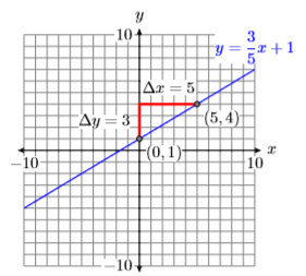
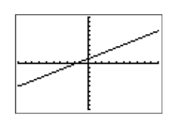
Cuando comparamos la imagen de la calculadora en Figura\(\PageIndex{3}\) con la gráfica dibujada a mano en Figura\(\PageIndex{2}\), obtenemos una mejor coincidencia.

Ejercicio\(\PageIndex{1}\)

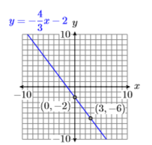
Dibuje la gráfica de la línea que tiene ecuación\(y=-\dfrac{4}{3} x-2\).

Contestar

Ejemplo\(\PageIndex{2}\)

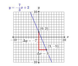
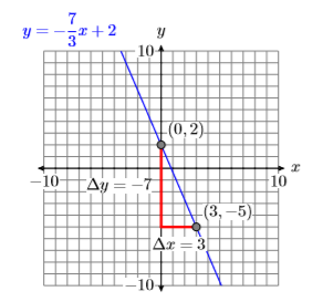
Dibuje la línea con\(y\) -intercepción\((0,2)\) y pendiente\(−7/3\). Etiquete la línea con la forma pendiente-intercepción de su ecuación.

Solución

Trazar la\(y\) -intercepción\((0,2)\). Ahora usa la pendiente\(−7/3\). Empezar en\((0,2)\), luego bajar siete unidades, seguido de un movimiento de tres unidades a la derecha al punto\((3,−5)\). Dibuja la línea a través de los puntos\((0,2)\) y\((3,−5)\). (Ver Figura\(\PageIndex{4}\)).

A continuación, la\(y\) -intercepción es\((0,2)\), entonces\(b = 2\). Además, la pendiente es\(−7/3\), entonces\(m = −7/3\). Sustituya estos números por la forma pendiente-intercepción de la línea.

\[\begin{aligned} y&= mx+b \quad \color {Red} \text { Slope-intercept form. } \\ y&= -\dfrac{7}{3} x+2 \quad \color {Red} \text { Substitute: }-7 / 3 \text { for } m, 2 \text { for } b . \end{aligned} \nonumber \]

Por lo tanto, la forma pendiente-intercepción de la línea es\(y=-\dfrac{7}{3} x+2\). Etiquete la línea con esta ecuación.

Figura\(\PageIndex{4}\): Gráfica dibujada a mano de\(y=-\dfrac{7}{3} x+2\)

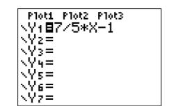
Comprobar: Para graficar\(y=-\dfrac{7}{3} x+2\), ingresa\(-7 / 3 * X+2\) Y1 en el menú Y =. Seleccione 6:ZStandard en el menú ZOOM, seguido de 5:ZSquare en el menú ZOOM para producir la gráfica que se muestra en la Figura\(\PageIndex{6}\).

Figura\(\PageIndex{5}\): Gráfica dibujada a mano de\(y=-\dfrac{7}{3} x+2\)

Figura\(\PageIndex{6}\): Seleccione 6:ZStandard en el menú ZOOM, seguido de 5:ZSquare en el menú ZOOM para producir la gráfica de la ecuación\(y=-\dfrac{7}{3} x+2\)

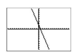
Esto proporciona una buena coincidencia del gráfico dibujado a mano en Figura\(\PageIndex{5}\) y nuestro resultado de calculadora gráfica en Figura\(\PageIndex{6}\).

Ejercicio\(\PageIndex{2}\)

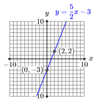
Dibuja la línea con\(y\)-intercept \((0,−3)\) and slope \(5/2\). Label the line with the slope-intercept form of its equation.

Contestar

Ejemplo\(\PageIndex{3}\)

Utilice la gráfica de la línea en la siguiente figura para encontrar la ecuación de la línea.

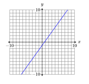
Solución

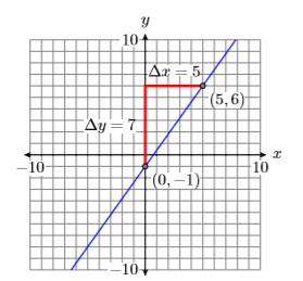
Tenga en cuenta que el\(y\)-intercept of the line is \((0,−1)\) (See Figure \(\PageIndex{7}\)). Next, we try to locate a point on the line that passes directly through a lattice point, a point where a vertical and horizontal grid line intersect. In Figure \(\PageIndex{7}\), we chose the point \((5,6)\). Now, starting at the \(y\)-intercept \((0,1)\), we move up \(7\) units, then to the right \(5\) units. Hence, the slope is \(m=\Delta y / \Delta x\), or \(m =7 /5\).

Note

We could also subtract the coordinates of point \((0,−1)\) from the coordinates of point \((5,6)\) to determine the slope. \[\dfrac{6-(-1)}{5-0}=\dfrac{7}{5} \nonumber \]

Figure \(\PageIndex{7}\): The line has \(y\)-intercept \((0,−1)\) and slope \(7/5\).

Next, state the slope-intercept form, the substitute \(7/5\) for \(m\) and \(−1\) for \(b\).

\[\begin{aligned} y&= mx+b \quad \color {Red} \text { Slope-intercept form. } \\ y&= \dfrac{7}{5} x+(-1) \quad \color {Red} \text { Substitute: } 7 / 5 \text { for } m,-1 \text { for } b \end{aligned} \nonumber \]

Thus, the equation of the line is \(y=\dfrac{7}{5} x-1\).

Check: This is an excellent situation to run a check on your graphing calculator.

Figure \(\PageIndex{8}\): Enter \(y=\dfrac{7}{5} x-1\) in the Y= menu.

Figure \(\PageIndex{9}\): Select 6:ZStandard followed by 5:ZSquare (both from the ZOOM menu) to produce this graph.

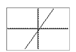
When we compare the result in Figure \(\PageIndex{9}\) with the original hand-drawn graph (see Figure \(\PageIndex{7}\)), we’re confident we have a good match.

Exercise \(\PageIndex{3}\)

Use the graph of the line in the figure below to find the equation of the line.

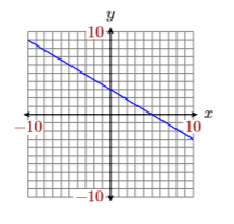
Answer

\(y=-\dfrac{3}{5} x+3\)

Applications

Let’s look at a linear application.

Example \(\PageIndex{4}\)

Jason spots his brother Tim talking with friends at the library, located \(300\) feet away. He begins walking towards his brother at a constant rate of \(2\) feet per second (\(2\) ft/s).

1. Express the distance \(d\) between Jason and his brother Tim in terms of the time \(t\).
2. At what time after Jason begins walking towards Tim are the brothers \(200\) feet apart?

Solution

Because the distance between Jason and his brother is decreasing at a constant rate, the graph of the distance versus time is a line. Let’s begin by making a rough sketch of the line. In Figure \(\PageIndex{10}\), note that we’ve labeled what are normally the \(x\)- and \(y\)-axes with the time \(t\) and distance \(d\), and we’ve included the units with our labels.

Figure \(\PageIndex{10}\): A plot of the distance \(d\) separating the brothers versus time \(t\).

Let \(t = 0\) seconds be the time that Jason begins walking towards his brother Tim. At time \(t = 0\), the initial distance between the brothers is \(300\) feet. This puts the \(d\)-intercept (normally the \(y\)-intercept) at the point \((0,300)\) (see Figure \(\PageIndex{10}\)).

Because Jason is walking toward his brother, the distance between the brothers decreases at a constant rate of \(2\) feet per second. This means the line must slant downhill, making the slope negative, so \(m = −2\) ft/s. We can construct an accurate plot of distance versus time by starting at the point \((0,300)\), then descending \(\Delta d=-300\), then moving to the right \(\Delta t=150\). This makes the slope \(\Delta d / \Delta t=-300 / 150=-2\) (See Figure \(\PageIndex{10}\)). Note that the slope is the rate at which the distance \(d\) between the brothers is changing with respect to time \(t\).

Finally, the equation of the line is \(y = mx + b\), where \(m\) is the slope of the line and \(b\) is the \(y\)-coordinate (in this case the \(d\)-coordinate) of the point where the graph crosses the vertical axis. Thus, substitute \(−2\) for \(m\), and \(300\) for \(b\) in the slope-intercept form of the line.

\[\begin{aligned} y&= mx+b \quad \color {Red} \text { Slope-intercept form. } \\ y&= -2x+300 \quad \color {Red} \text { Substitute: }-2 \text { for } m, 300 \text { for } b \end{aligned} \nonumber \]

One problem remains. The equation \(y = −2x + 300\) gives us \(y\) in terms of \(x\).

1. The question required that we express the distance \(d\) in terms of the time \(t\). So, to finish the solution, replace \(y\) with \(d\) and \(x\) with \(t\) (check the axes labels in Figure \(\PageIndex{10}\)) to obtain a solution: \[d=-2t+300 \nonumber \]
2. Now that our equation expresses the distance between the brothers in terms of time, let’s answer part (b), “At what time after Jason begins walking towards Tim are the brothers \(200\) feet apart?” To find this time, substitute \(200\) for \(d\) in the equation \(d =−2t + 300\), then solve for \(t\).\[\begin{aligned} d &= -2t+300 \quad \color {Red} \text { Distance equation } \\ 200 &= -2t+300 \quad \color {Red} \text { Substitute } 200 \text { for } d \end{aligned} \nonumber \]Solve this last equation for the time \(t\).\[\begin{aligned} 200-300&= -2t+300-300 \quad \color {Red} \text { Subtract } 300 \text { from both sides. } \\ -100&= -2t \quad \color {Red} \text { Simplify both sides. } \\ \dfrac{-100}{-2}&= \dfrac{-2 t}{-2} \quad \color {Red} \text { Divide both sides by }-2 \\ 50&= t \quad \color {Red} \text { Simplify both sides. } \end{aligned} \nonumber \]Thus, it takes Jason \(50\) seconds to close the distance between the brothers to \(200\) feet.

Exercise \(\PageIndex{4}\)

A swimmer is \(50\) feet from the beach, and then begins swimming away from the beach at a constant rate of \(1.5\) feet per second (\(1.5\) ft/s). Express the distance \(d\) between the swimmer and the beach in terms of the time \(t\).

Answer

\(d=1.5 t+50\)