
6.5: El Método de los Mínimos Cuadrados
- Page ID
- 113086
- Conoce ejemplos de problemas de mejor ajuste.
- Aprende a convertir un problema de mejor ajuste en un problema de mínimos cuadrados.
- Receta: encontrar una solución de mínimos cuadrados (de dos maneras). solución.
- Imagen: geometría de una solución de mínimos cuadrados.
- Palabras de vocabulario: solución de mínimos cuadrados.
En esta sección, respondemos a la siguiente pregunta importante:
Supongamos que\(Ax=b\) no tiene solución. ¿Cuál es la mejor solución aproximada?
Para nuestros propósitos, la mejor solución aproximada se llama la solución de mínimos cuadrados. Presentaremos dos métodos para encontrar soluciones de mínimos cuadrados, y daremos varias aplicaciones a los problemas de mejor ajuste.
Soluciones de mínimos cuadrados
Comenzamos aclarando exactamente qué queremos decir con una “mejor solución aproximada” a una ecuación matricial inconsistente\(Ax=b\).
Dejar\(A\) ser una\(m\times n\) matriz y dejar\(b\) ser un vector en\(\mathbb{R}^m \). Una solución de mínimos cuadrados de la ecuación matricial\(Ax=b\) es un vector de\(\mathbb{R}^n \) tal\(\hat x\) manera que
\[ \text{dist}(b,\,A\hat x) \leq \text{dist}(b,\,Ax) \nonumber \]
para todos los demás vectores\(x\) en\(\mathbb{R}^n \).
Recordemos que\(\text{dist}(v,w) = \|v-w\|\) es la distancia, Definición 6.1.2 en la Sección 6.1, entre los vectores\(v\) y\(w\). El término “mínimos cuadrados” proviene del hecho de que\(\text{dist}(b,Ax) = \|b-A\hat x\|\) es la raíz cuadrada de la suma de los cuadrados de las entradas del vector\(b-A\hat x\). Entonces una solución de mínimos cuadrados minimiza la suma de los cuadrados de las diferencias entre las entradas de\(A\hat x\) y\(b\). Es decir, una solución de mínimos cuadrados resuelve la ecuación lo más cerca\(Ax=b\) posible, en el sentido de que\(b-Ax\) se minimiza la suma de los cuadrados de la diferencia.
Mínimos Cuadrados: Imagen
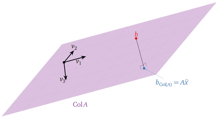
Supongamos que la ecuación\(Ax=b\) es inconsistente. Recordemos de la Nota 2.3.6 en la Sección 2.3 que el espacio de columna de\(A\) es el conjunto de todos los demás vectores\(c\) tal que\(Ax=c\) es consistente. En otras palabras,\(\text{Col}(A)\) es el conjunto de todos los vectores de la forma\(Ax.\) De ahí, el vector más cercano, Nota 6.3.1 en la Sección 6.3, de la forma\(Ax\) a\(b\) es la proyección ortogonal de\(b\) sobre\(\text{Col}(A)\). Esto se denota\(b_{\text{Col}(A)}\text{,}\) siguiendo la Definición 6.3.1 en la Sección 6.3.
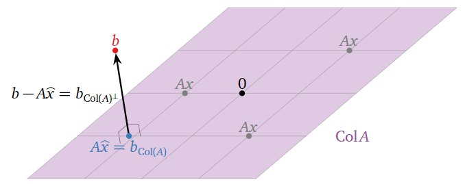
Figura\(\PageIndex{1}\)
Una solución de mínimos cuadrados de\(Ax=b\) es una solución\(\hat x\) de la ecuación consistente\(Ax=b_{\text{Col}(A)}\)
Si\(Ax=b\) es consistente,\(b_{\text{Col}(A)} = b\text{,}\) entonces para que una solución de mínimos cuadrados sea la misma que una solución habitual.
¿Dónde está\(\hat x\) en esta imagen? Si\(v_1,v_2,\ldots,v_n\) son las columnas de\(A\text{,}\) entonces
\[ A\hat x = A\left(\begin{array}{c}\hat{x}_1 \\ \hat{x}_2 \\ \vdots \\ \hat{x}_{n}\end{array}\right) = \hat x_1v_1 + \hat x_2v_2 + \cdots + \hat x_nv_n. \nonumber \]
De ahí que las entradas de\(\hat x\) sean las “coordenadas” de\(b_{\text{Col}(A)}\) con respecto al conjunto\(\{v_1,v_2,\ldots,v_m\}\) de expansión de\(\text{Col}(A)\). (Son honestos\(\mathcal{B}\) -coordenadas si las columnas de\(A\) son linealmente independientes.)
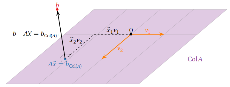
Figura\(\PageIndex{2}\)
Aprendimos a resolver este tipo de problema de proyección ortogonal en la Sección 6.3.
Dejar\(A\) ser una\(m\times n\) matriz y dejar\(b\) ser un vector en\(\mathbb{R}^m \). Las soluciones de mínimos cuadrados de\(Ax=b\) son las soluciones de la ecuación matricial
\[ A^TAx = A^Tb \nonumber \]
- Prueba
-
Por Teorema 6.3.2 en la Sección 6.3, si\(\hat x\) es una solución de la ecuación matricial\(A^TAx = A^Tb\text{,}\) entonces\(A\hat x\) es igual a\(b_{\text{Col}(A)}\). Argumentamos anteriormente que una solución de mínimos cuadrados de\(Ax=b\) es una solución de\(Ax = b_{\text{Col}(A)}.\)
En particular, encontrar una solución de mínimos cuadrados significa resolver un sistema consistente de ecuaciones lineales. Podemos traducir el teorema anterior en una receta:
Dejar\(A\) ser una\(m\times n\) matriz y dejar\(b\) ser un vector en\(\mathbb{R}^n \). Aquí hay un método para calcular una solución de mínimos cuadrados de\(Ax=b\text{:}\)
- Calcular la matriz\(A^TA\) y el vector\(A^Tb\).
- Formar la matriz aumentada para la ecuación matricial\(A^TAx = A^Tb\text{,}\) y reducir la fila.
- Esta ecuación siempre es consistente, y cualquier solución\(\hat x\) es una solución de mínimos cuadrados.
Para reiterar: una vez que haya encontrado una solución\(\hat x\) de mínimos cuadrados de\(Ax=b\text{,}\) entonces\(b_{\text{Col}(A)}\) es igual a\(A\hat x\).
Encuentre las soluciones de mínimos cuadrados de\(Ax=b\) dónde:
\[ A = \left(\begin{array}{cc}0&1\\1&1\\2&1\end{array}\right) \qquad b = \left(\begin{array}{c}6\\0\\0\end{array}\right). \nonumber \]
¿Qué cantidad se está minimizando?
Solución
Tenemos
\[ A^TA = \left(\begin{array}{ccc}0&1&2\\1&1&1\end{array}\right)\left(\begin{array}{cc}0&1\\1&1\\2&1\end{array}\right) = \left(\begin{array}{cc}5&3\\3&3\end{array}\right) \nonumber \]
y
\[ A^T b = \left(\begin{array}{ccc}0&1&2\\1&1&1\end{array}\right)\left(\begin{array}{c}6\\0\\0\end{array}\right) = \left(\begin{array}{c}0\\6\end{array}\right). \nonumber \]
Formamos una matriz aumentada y la fila reducimos:
\[ \left(\begin{array}{cc|c}5&3&0\\3&3&6\end{array}\right)\xrightarrow{\text{RREF}}\left(\begin{array}{cc|c}1&0&-3\\0&1&5\end{array}\right). \nonumber \]
Por lo tanto, la única solución de mínimos cuadrados es\(\hat x = {-3\choose 5}.\)
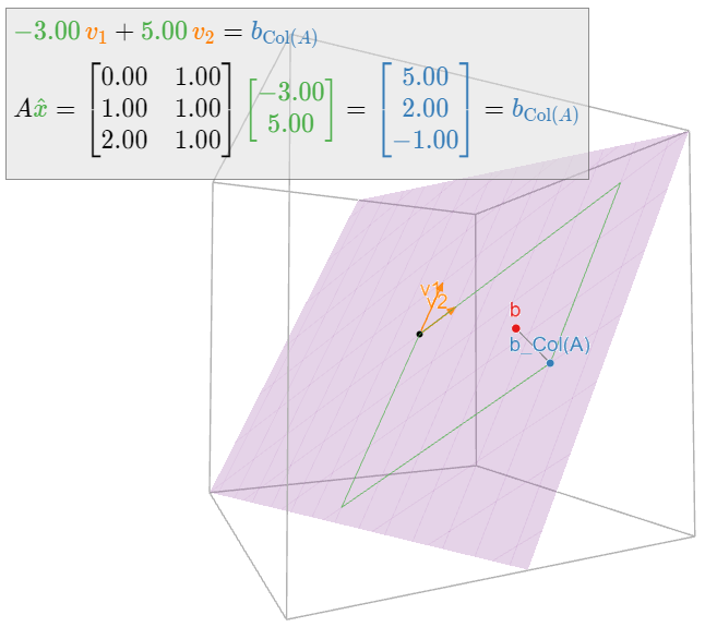
Esta solución minimiza la distancia de\(A\hat x\) a\(b\text{,}\) es decir, la suma de los cuadrados de las entradas de\(b-A\hat x = b-b_{\text{Col}(A)} = b_{\text{Col}(A)^\perp}\). En este caso, tenemos
\[||b-A\hat{x}||=\left|\left|\left(\begin{array}{c}6\\0\\0\end{array}\right)-\left(\begin{array}{c}5\\2\\-1\end{array}\right)\right|\right|=\left|\left|\left(\begin{array}{c}1\\-2\\1\end{array}\right)\right|\right|=\sqrt{1^2+(-2)^2+1^2}=\sqrt{6}.\nonumber\]
Por lo tanto,\(b_{\text{Col}(A)} = A\hat x\) es\(\sqrt 6\) unidades de\(b.\)
En la siguiente imagen,\(v_1,v_2\) se encuentran las columnas de\(A\text{:}\)
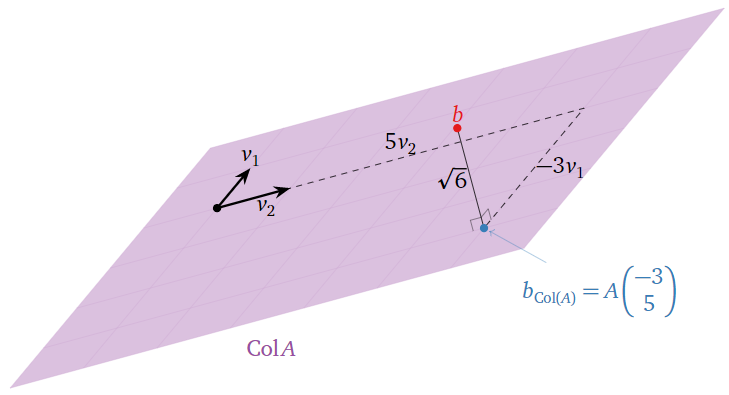
Figura\(\PageIndex{4}\)
Encuentre las soluciones de mínimos cuadrados de\(Ax=b\) dónde:
\[ A = \left(\begin{array}{cc}2&0\\-1&1\\0&2\end{array}\right) \qquad b = \left(\begin{array}{c}1\\0\\-1\end{array}\right). \nonumber \]
Solución
Tenemos
\[ A^T A = \left(\begin{array}{ccc}2&-1&0\\0&1&2\end{array}\right)\left(\begin{array}{cc}2&0\\-1&1\\0&2\end{array}\right) = \left(\begin{array}{cc}5&-1\\-1&5\end{array}\right) \nonumber \]
y
\[ A^T b = \left(\begin{array}{ccc}2&-1&0\\0&1&2\end{array}\right)\left(\begin{array}{c}1\\0\\-1\end{array}\right) = \left(\begin{array}{c}2\\-2\end{array}\right). \nonumber \]
Formamos una matriz aumentada y la fila reducimos:
\[ \left(\begin{array}{cc|c}5&-1&2\\-1&5&-2\end{array}\right)\xrightarrow{\text{RREF}}\left(\begin{array}{cc|c}1&0&1/3\\0&1&-1/3\end{array}\right). \nonumber \]
Por lo tanto, la única solución de mínimos cuadrados es\(\hat x = \frac 13{1\choose -1}.\)
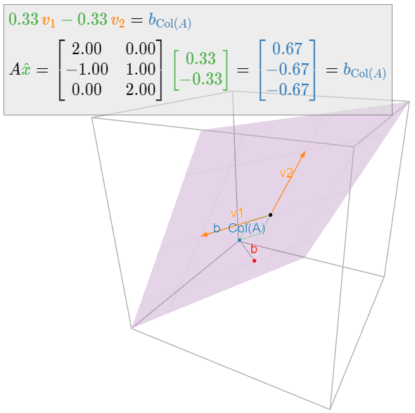
El lector puede haber notado que hemos tenido cuidado de decir “las soluciones de mínimos cuadrados” en plural, y “una solución de mínimos cuadrados” usando el artículo indefinido. Esto se debe a que una solución de mínimos cuadrados no necesita ser única: de hecho, si las columnas de\(A\) son linealmente dependientes, entonces\(Ax=b_{\text{Col}(A)}\) tiene infinitamente muchas soluciones. El siguiente teorema, que da criterios equivalentes de singularidad, es un análogo del Corolario 6.3.1 en la Sección 6.3.
Dejar\(A\) ser una\(m\times n\) matriz y dejar\(b\) ser un vector en\(\mathbb{R}^m \). Los siguientes son equivalentes:
- \(Ax=b\)tiene una solución única de mínimos cuadrados.
- Las columnas de\(A\) son linealmente independientes.
- \(A^TA\)es invertible.
En este caso, la solución de mínimos cuadrados es
\[ \hat x = (A^TA)^{-1} A^Tb. \nonumber \]
- Prueba
-
El conjunto de soluciones de mínimos cuadrados de\(Ax=b\) es el conjunto de soluciones de la ecuación consistente\(A^TAx=A^Tb\text{,}\) que es una traducción del conjunto de soluciones de la ecuación homogénea\(A^TAx=0\). Dado que\(A^TA\) es una matriz cuadrada, la equivalencia de 1 y 3 se desprende del Teorema 5.1.1 en la Sección 5.1. El conjunto de soluciones de mínimos cuadrados es también el conjunto de soluciones de la ecuación consistente\(Ax = b_{\text{Col}(A)}\text{,}\) que tiene una solución única si y solo si las columnas de\(A\) son linealmente independientes por Receta: Comprobación de Independencia Lineal en la Sección 2.5.
Encuentre las soluciones de mínimos cuadrados de\(Ax=b\) dónde:
\[ A = \left(\begin{array}{ccc}1&0&1\\1&1&-1\\1&2&-3\end{array}\right) \qquad b = \left(\begin{array}{c}6\\0\\0\end{array}\right). \nonumber \]
Solución
Tenemos
\[ A^TA = \left(\begin{array}{ccc}3&3&-3\\3&5&-7\\-3&-7&11\end{array}\right) \qquad A^Tb = \left(\begin{array}{c}6\\0\\6\end{array}\right). \nonumber \]
Formamos una matriz aumentada y la fila reducimos:
\[ \left(\begin{array}{ccc|c}3&3&-3&6\\3&5&-7&0\\-3&-7&11&6\end{array}\right)\xrightarrow{\text{RREF}}\left(\begin{array}{ccc|c}1&0&1&5\\0&1&-2&-3\\0&0&0&0\end{array}\right). \nonumber \]
La variable libre es\(x_3\text{,}\) así que el conjunto de soluciones es
\[\left\{\begin{array}{rrrrr}x_1 &=& -x_3 &+& 5\\ x_2 &=& 2x_3 &-& 3\\ x_3 &=& x_3&{}&{}\end{array}\right. \quad\xrightarrow[\text{vector form}]{\text{parametric}}\quad \hat{x}=\left(\begin{array}{c}x_1\\x_2\\x_3\end{array}\right)=x_3\left(\begin{array}{c}-1\\2\\1\end{array}\right)+\left(\begin{array}{c}5\\-3\\0\end{array}\right).\nonumber\]
Por ejemplo, tomando\(x_3 = 0\) y\(x_3=1\) da las soluciones de mínimos cuadrados
\[ \hat x = \left(\begin{array}{c}5\\-3\\0\end{array}\right)\quad\text{and}\quad \hat x =\left(\begin{array}{c}4\\-1\\1\end{array}\right). \nonumber \]
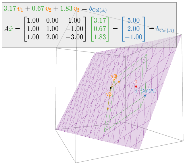
Geométricamente, vemos que las columnas\(v_1,v_2,v_3\) de\(A\) son coplanares:
Figura\(\PageIndex{7}\)
Por lo tanto, hay muchas formas de escribir\(b_{\text{Col}(A)}\) como una combinación lineal de\(v_1,v_2,v_3\).
Como es habitual, los cálculos que involucran proyecciones se vuelven más fáciles en presencia de un conjunto ortogonal. En efecto, si\(A\) es una\(m\times n\) matriz con columnas ortogonales\(u_1,u_2,\ldots,u_m\text{,}\) entonces podemos usar el Teorema 6.4.1 en la Sección 6.4 para escribir
\[ b_{\text{Col}(A)} = \frac{b\cdot u_1}{u_1\cdot u_1}\,u_1 + \frac{b\cdot u_2}{u_2\cdot u_2}\,u_2 + \cdots + \frac{b\cdot u_m}{u_m\cdot u_m}\,u_m = A\left(\begin{array}{c}(b\cdot u_1)/(u_1\cdot u_1) \\ (b\cdot u_2)/(u_2\cdot u_2) \\ \vdots \\ (b\cdot u_m)/(u_m\cdot u_m)\end{array}\right). \nonumber \]
Obsérvese que la solución de mínimos cuadrados es única en este caso, ya que un conjunto ortogonal es linealmente independiente, Fact 6.4.1 en la Sección 6.4.
Dejar\(A\) ser una\(m\times n\) matriz con columnas ortogonales\(u_1,u_2,\ldots,u_m\text{,}\) y dejar\(b\) ser un vector en\(\mathbb{R}^n \). Entonces la solución de mínimos cuadrados de\(Ax=b\) es el vector
\[ \hat x = \left(\frac{b\cdot u_1}{u_1\cdot u_1},\; \frac{b\cdot u_2}{u_2\cdot u_2},\; \ldots,\; \frac{b\cdot u_m}{u_m\cdot u_m} \right). \nonumber \]
Esta fórmula es particularmente útil en las ciencias, ya que las matrices con columnas ortogonales a menudo surgen en la naturaleza.
Encuentre la solución de mínimos cuadrados de\(Ax=b\) dónde:
\[ A = \left(\begin{array}{ccc}1&0&1\\0&1&1\\-1&0&1\\0&-1&1\end{array}\right) \qquad b = \left(\begin{array}{c}0\\1\\3\\4\end{array}\right). \nonumber \]
Solución
\(u_1,u_2,u_3\)Dejen ser las columnas de\(A\). Estos forman un conjunto ortogonal, por lo que
\[ \hat x = \left(\frac{b\cdot u_1}{u_1\cdot u_1},\; \frac{b\cdot u_2}{u_2\cdot u_2},\; \frac{b\cdot u_3}{u_3\cdot u_3} \right) = \left(\frac{-3}{2},\;\frac{-3}{2},\;\frac{8}{4}\right) = \left(-\frac32,\;-\frac32,\;2\right). \nonumber \]
Compare el Ejemplo 6.4.8 en la Sección 6.4.
Problemas de mejor ajuste
En esta subsección damos una aplicación del método de mínimos cuadrados al modelado de datos. Comenzamos con un ejemplo básico.
Supongamos que hemos medido tres puntos de datos
\[ (0,6),\quad (1,0),\quad (2,0), \nonumber \]
y que nuestro modelo para estos datos asevera que los puntos deben estar en una línea. Por supuesto, estos tres puntos en realidad no se encuentran en una sola línea, pero esto podría deberse a errores en nuestra medición. ¿Cómo predecimos en qué línea se supone que deben acostarse?
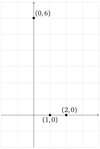
Figura\(\PageIndex{9}\)
La ecuación general para una línea (no vertical) es
\[ y = Mx + B. \nonumber \]
Si nuestros tres puntos de datos estuvieran en esta línea, entonces se cumplirían las siguientes ecuaciones:
\[\begin{align} 6&=M\cdot 0+B\nonumber \\ 0&=M\cdot 1+B\label{eq:1} \\ 0&=M\cdot 2+B.\nonumber\end{align}\]
Para encontrar la línea de mejor ajuste, tratamos de resolver las ecuaciones anteriores en las incógnitas\(M\) y\(B\). Como los tres puntos en realidad no se encuentran en una línea, no hay una solución real, así que en su lugar calculamos una solución de mínimos cuadrados.
Poniendo nuestras ecuaciones lineales en forma de matriz, estamos tratando de resolver\(Ax=b\) para
\[ A = \left(\begin{array}{cc}0&1\\1&1\\2&1\end{array}\right) \qquad x = \left(\begin{array}{c}M\\B\end{array}\right)\qquad b = \left(\begin{array}{c}6\\0\\0\end{array}\right). \nonumber \]
Resolvimos este problema de mínimos cuadrados en Ejemplo\(\PageIndex{1}\): la única solución de mínimos cuadrados\(Ax=b\) es\(\hat x = {M\choose B} = {-3\choose 5}\text{,}\) así que la línea de mejor ajuste es
\[ y = -3x + 5. \nonumber \]
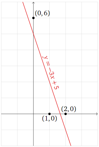
Figura\(\PageIndex{10}\)
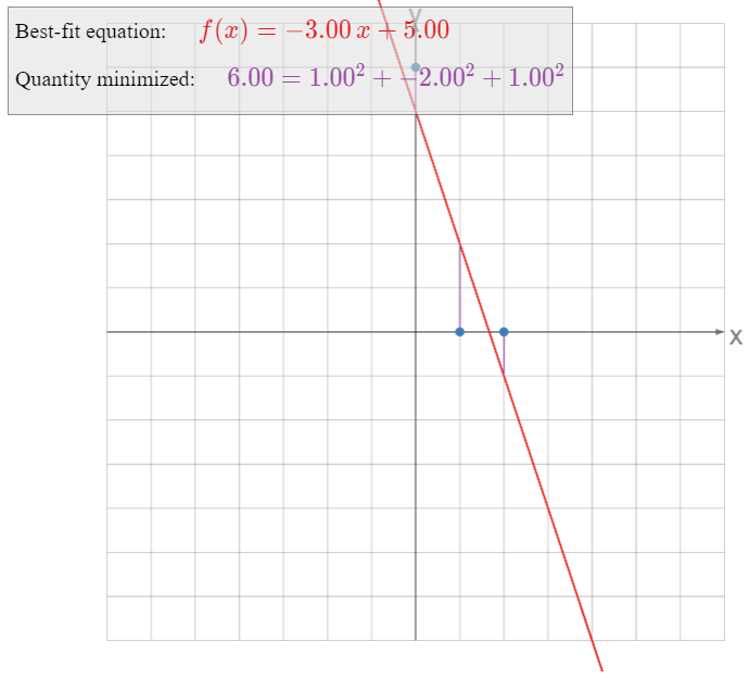
¿Qué es exactamente la línea\(y= f(x) = -3x+5\) minimizando? La solución de mínimos cuadrados\(\hat x\) minimiza la suma de los cuadrados de las entradas del vector\(b-A\hat x\). El vector\(b\) es el lado izquierdo de\(\eqref{eq:1}\), y
\[ A\left(\begin{array}{c}-3\\5\end{array}\right) = \left(\begin{array}{c}-3(0)+5\\-3(1)+5\\-3(2)+5\end{array}\right) = \left(\begin{array}{c}f(0)\\f(1)\\f(2)\end{array}\right). \nonumber \]
En otras palabras,\(A\hat x\) es el vector cuyas entradas son las\(y\) -coordenadas de la gráfica de la línea en los valores de\(x\) que especificamos en nuestros puntos de datos, y\(b\) es el vector cuyas entradas son las\(y\) -coordenadas de esos puntos de datos. La diferencia\(b-A\hat x\) es la distancia vertical de la gráfica desde los puntos de datos:
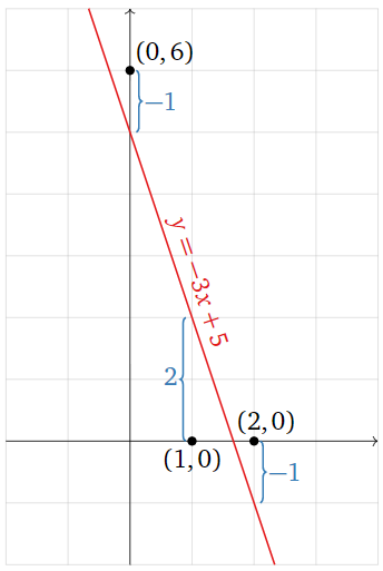
Figura\(\PageIndex{11}\)
\[\color{blue}{b-A\hat{x}=\left(\begin{array}{c}6\\0\\0\end{array}\right)-A\left(\begin{array}{c}-3\\5\end{array}\right)=\left(\begin{array}{c}-1\\2\\-1\end{array}\right)}\nonumber\]
La línea de mejor ajuste minimiza la suma de los cuadrados de estas distancias verticales.
Find the parabola that best approximates the data points
\[ (-1,\,1/2),\quad(1,\,-1),\quad(2,\,-1/2),\quad(3,\,2). \nonumber \]

Figure \(\PageIndex{13}\)
What quantity is being minimized?
Solution
The general equation for a parabola is
\[ y = Bx^2 + Cx + D. \nonumber \]
If the four points were to lie on this parabola, then the following equations would be satisfied:
\[\begin{align} \frac{1}{2}&=B(-1)^2+C(-1)+D\nonumber \\ -1&=B(1)^2+C(1)+D\nonumber \\ -\frac{1}{2}&=B(2)^2+C(2)+D\label{eq:2} \\ 2&=B(3)^2+C(3)+D.\nonumber\end{align}\]
We treat this as a system of equations in the unknowns \(B,C,D\). In matrix form, we can write this as \(Ax=b\) for
\[ A = \left(\begin{array}{ccc}1&-1&1\\1&1&1\\4&2&1\\9&3&1\end{array}\right) \qquad x = \left(\begin{array}{c}B\\C\\D\end{array}\right) \qquad b = \left(\begin{array}{c}1/2 \\ -1\\-1/2 \\ 2\end{array}\right). \nonumber \]
We find a least-squares solution by multiplying both sides by the transpose:
\[ A^TA = \left(\begin{array}{ccc}99&35&15\\35&15&5\\15&5&4\end{array}\right) \qquad A^Tb = \left(\begin{array}{c}31/2\\7/2\\1\end{array}\right), \nonumber \]
then forming an augmented matrix and row reducing:
\[ \left(\begin{array}{ccc|c}99&35&15&31/2 \\ 35&15&5&7/2 \\ 15&5&4&1\end{array}\right)\xrightarrow{\text{RREF}}\left(\begin{array}{ccc|c}1&0&0&53/88 \\ 0&1&0&-379/440 \\ 0&0&1&-41/44\end{array}\right) \implies \hat x = \left(\begin{array}{c}53/88 \\ -379/440 \\ -41/44 \end{array}\right). \nonumber \]
The best-fit parabola is
\[ y = \frac{53}{88}x^2 - \frac{379}{440}x - \frac{41}{44}. \nonumber \]
Multiplying through by \(88\text{,}\) we can write this as
\[ 88y = 53x^2 - \frac{379}{5}x - 82. \nonumber \]
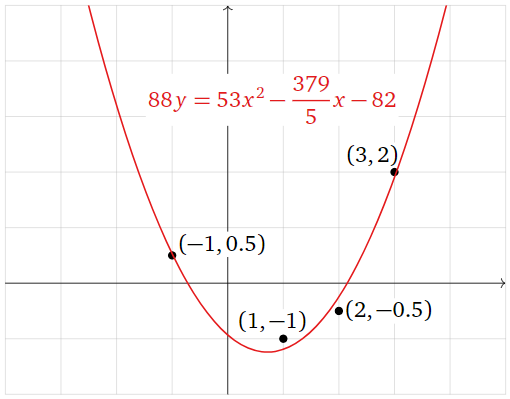
Figure \(\PageIndex{14}\)
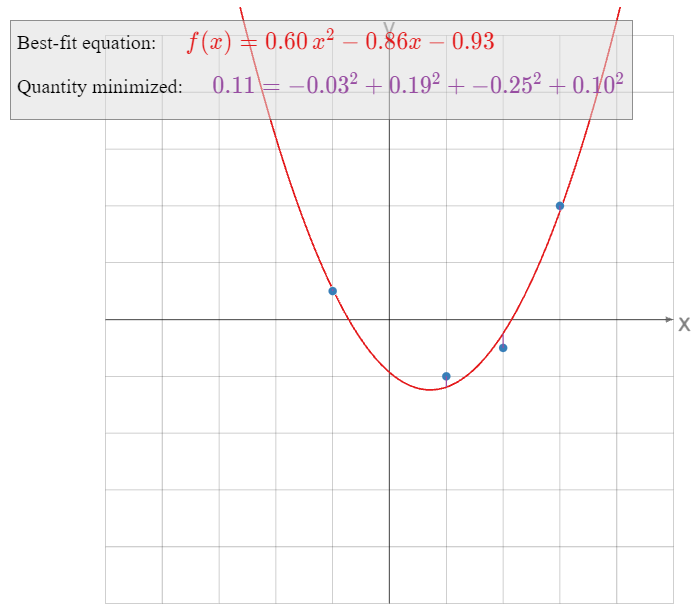
Now we consider what exactly the parabola \(y = f(x)\) is minimizing. The least-squares solution \(\hat x\) minimizes the sum of the squares of the entries of the vector \(b-A\hat x\). The vector \(b\) is the left-hand side of \(\eqref{eq:2}\), and
\[A\hat{x}=\left(\begin{array}{c} \frac{53}{88}(-1)^2-\frac{379}{440}(-1)-\frac{41}{44} \\ \frac{53}{88}(1)^2-\frac{379}{440}(1)-\frac{41}{44} \\ \frac{53}{88}(2)^2-\frac{379}{440}(2)-\frac{41}{44} \\ \frac{53}{88}(3)^2-\frac{379}{440}(3)-\frac{41}{44}\end{array}\right)=\left(\begin{array}{c}f(-1) \\ f(1) \\ f(2) \\ f(3)\end{array}\right).\nonumber\]
In other words, \(A\hat x\) is the vector whose entries are the \(y\)-coordinates of the graph of the parabola at the values of \(x\) we specified in our data points, and \(b\) is the vector whose entries are the \(y\)-coordinates of those data points. The difference \(b-A\hat x\) is the vertical distance of the graph from the data points:
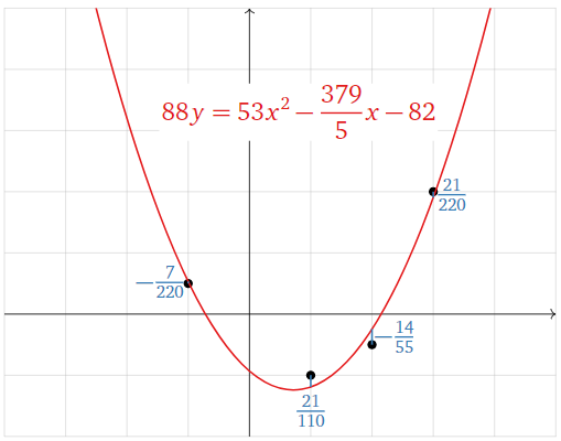
Figure \(\PageIndex{15}\)
\[\color{blue}{b-A\hat{x}=\left(\begin{array}{c}1/2 \\ -1 \\ -1/2 \\ 2\end{array}\right)-A\left(\begin{array}{c}53/88 \\ -379/440 \\ -41/44\end{array}\right)=\left(\begin{array}{c}-7/220 \\ 21/110 \\ -14/55 \\ 21/220\end{array}\right)}\nonumber\]
The best-fit parabola minimizes the sum of the squares of these vertical distances.
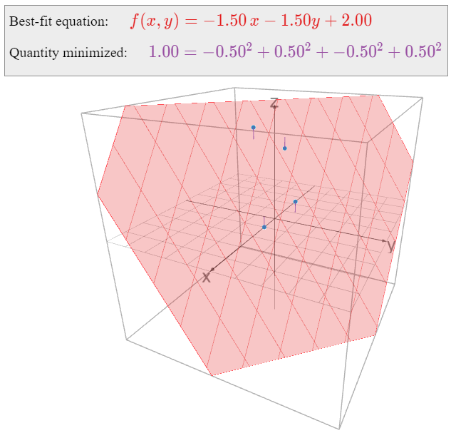
Find the linear function \(f(x,y)\) that best approximates the following data:
\[ \begin{array}{r|r|c} x & y & f(x,y) \\\hline 1 & 0 & 0 \\ 0 & 1 & 1 \\ -1 & 0 & 3 \\ 0 & -1 & 4 \end{array} \nonumber \]
What quantity is being minimized?
Solution
The general equation for a linear function in two variables is
\[ f(x,y) = Bx + Cy + D. \nonumber \]
We want to solve the following system of equations in the unknowns \(B,C,D\text{:}\)
\[\begin{align} B(1)+C(0)+D&=0 \nonumber \\ B(0)+C(1)+D&=1 \nonumber \\ B(-1)+C(0)+D&=3\label{eq:3} \\ B(0)+C(-1)+D&=4\nonumber\end{align}\]
In matrix form, we can write this as \(Ax=b\) for
\[ A = \left(\begin{array}{ccc}1&0&1\\0&1&1\\-1&0&1\\0&-1&1\end{array}\right) \qquad x = \left(\begin{array}{c}B\\C\\D\end{array}\right) \qquad b = \left(\begin{array}{c}0\\1\\3\\4\end{array}\right). \nonumber \]
We observe that the columns \(u_1,u_2,u_3\) of \(A\) are orthogonal, so we can use Recipe 2: Compute a Least-Squares Solution:
\[ \hat x = \left(\frac{b\cdot u_1}{u_1\cdot u_1},\; \frac{b\cdot u_2}{u_2\cdot u_2},\; \frac{b\cdot u_3}{u_3\cdot u_3} \right) = \left(\frac{-3}{2},\;\frac{-3}{2},\;\frac{8}{4}\right) = \left(-\frac32,\;-\frac32,\;2\right). \nonumber \] We find a least-squares solution by multiplying both sides by the transpose:
\[ A^TA = \left(\begin{array}{ccc}2&0&0\\0&2&0\\0&0&4\end{array}\right) \qquad A^Tb = \left(\begin{array}{c}-3\\-3\\8\end{array}\right). \nonumber \] The matrix \(A^TA\) is diagonal (do you see why that happened?), so it is easy to solve the equation \(A^TAx = A^Tb\text{:}\)
\[ \left(\begin{array}{cccc}2&0&0&-3 \\ 0&2&0&-3 \\ 0&0&4&8\end{array}\right) \xrightarrow{\text{RREF}} \left(\begin{array}{cccc}1&0&0&-3/2 \\ 0&1&0&-3/2 \\ 0&0&1&2\end{array}\right) \implies \hat x = \left(\begin{array}{c}-3/2 \\ -3/2 \\ 2\end{array}\right). \nonumber \] Therefore, the best-fit linear equation is
\[ f(x,y) = -\frac 32x - \frac32y + 2. \nonumber \]
Here is a picture of the graph of \(f(x,y)\text{:}\)
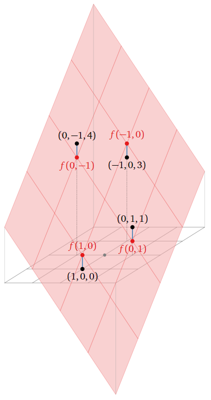
Figure \(\PageIndex{17}\)
Now we consider what quantity is being minimized by the function \(f(x,y)\). The least-squares solution \(\hat x\) minimizes the sum of the squares of the entries of the vector \(b-A\hat x\). The vector \(b\) is the right-hand side of \(\eqref{eq:3}\), and
\[A\hat{x}=\left(\begin{array}{rrrrr}-\frac32(1) &-& \frac32(0) &+& 2\\ -\frac32(0) &-& \frac32(1) &+& 2\\ -\frac32(-1) &-& \frac32(0) &+& 2\\ -\frac32(0) &-& \frac32(-1) &+& 2\end{array}\right)=\left(\begin{array}{c}f(1,0) \\ f(0,1) \\ f(-1,0) \\ f(0,-1)\end{array}\right).\nonumber\]
In other words, \(A\hat x\) is the vector whose entries are the values of \(f\) evaluated on the points \((x,y)\) we specified in our data table, and \(b\) is the vector whose entries are the desired values of \(f\) evaluated at those points. The difference \(b-A\hat x\) is the vertical distance of the graph from the data points, as indicated in the above picture. The best-fit linear function minimizes the sum of these vertical distances.
All of the above examples have the following form: some number of data points \((x,y)\) are specified, and we want to find a function
\[ y = B_1g_1(x) + B_2g_2(x) + \cdots + B_mg_m(x) \nonumber \]
that best approximates these points, where \(g_1,g_2,\ldots,g_m\) are fixed functions of \(x\). Indeed, in the best-fit line example we had \(g_1(x)=x\) and \(g_2(x)=1\text{;}\) in the best-fit parabola example we had \(g_1(x)=x^2\text{,}\) \(g_2(x)=x\text{,}\) and \(g_3(x)=1\text{;}\) and in the best-fit linear function example we had \(g_1(x_1,x_2)=x_1\text{,}\) \(g_2(x_1,x_2)=x_2\text{,}\) and \(g_3(x_1,x_2)=1\) (in this example we take \(x\) to be a vector with two entries). We evaluate the above equation on the given data points to obtain a system of linear equations in the unknowns \(B_1,B_2,\ldots,B_m\)—once we evaluate the \(g_i\text{,}\) they just become numbers, so it does not matter what they are—and we find the least-squares solution. The resulting best-fit function minimizes the sum of the squares of the vertical distances from the graph of \(y = f(x)\) to our original data points.
To emphasize that the nature of the functions \(g_i\) really is irrelevant, consider the following example.
What is the best-fit function of the form
\[ y=B+C\cos(x)+D\sin(x)+E\cos(2x)+F\sin(2x)+G\cos(3x)+H\sin(3x) \nonumber \]
passing through the points
\[ \left(\begin{array}{c}-4\\ -1\end{array}\right),\; \left(\begin{array}{c}-3\\ 0\end{array}\right),\; \left(\begin{array}{c}-2\\ -1.5\end{array}\right),\; \left(\begin{array}{c}-1\\ .5\end{array}\right),\; \left(\begin{array}{c}0\\1\end{array}\right),\; \left(\begin{array}{c}1\\-1\end{array}\right),\; \left(\begin{array}{c}2\\-.5\end{array}\right),\; \left(\begin{array}{c}3\\2\end{array}\right),\; \left(\begin{array}{c}4 \\-1\end{array}\right)? \nonumber \]
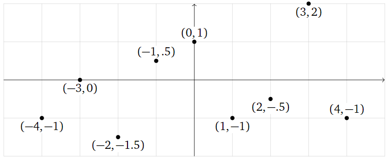
Figure \(\PageIndex{19}\)
Solution
We want to solve the system of equations
\[\begin{array}{rrrrrrrrrrrrrrr} -1 &=& B &+& C\cos(-4) &+& D\sin(-4) &+& E\cos(-8) &+& F\sin(-8) &+& G\cos(-12) &+& H\sin(-12)\\ 0 &=& B &+& C\cos(-3) &+& D\sin(-3) &+& E\cos(-6) &+& F\sin(-6) &+& G\cos(-9) &+& H\sin(-9)\\ -1.5 &=& B &+& C\cos(-2) &+& D\sin(-2) &+& E\cos(-4) &+& F\sin(-4) &+& G\cos(-6) &+& H\sin(-6) \\ 0.5 &=& B &+& C\cos(-1) &+& D\sin(-1) &+& E\cos(-2) &+& F\sin(-2) &+& G\cos(-3) &+& H\sin(-3)\\ 1 &=& B &+& C\cos(0) &+& D\sin(0) &+& E\cos(0) &+& F\sin(0) &+& G\cos(0) &+& H\sin(0)\\ -1 &=& B &+& C\cos(1) &+& D\sin(1) &+& E\cos(2) &+& F\sin(2) &+& G\cos(3) &+& H\sin(3)\\ -0.5 &=& B &+& C\cos(2) &+& D\sin(2) &+& E\cos(4) &+& F\sin(4) &+& G\cos(6) &+& H\sin(6)\\ 2 &=& B &+& C\cos(3) &+& D\sin(3) &+& E\cos(6) &+& F\sin(6) &+& G\cos(9) &+& H\sin(9)\\ -1 &=& B &+& C\cos(4) &+& D\sin(4) &+& E\cos(8) &+& F\sin(8) &+& G\cos(12) &+& H\sin(12).\end{array}\nonumber\]
All of the terms in these equations are numbers, except for the unknowns \(B,C,D,E,F,G,H\text{:}\)
\[\begin{array}{rrrrrrrrrrrrrrr} -1 &=& B &-& 0.6536C &+& 0.7568D &-& 0.1455E &-& 0.9894F &+& 0.8439G &+& 0.5366H\\ 0 &=& B &-& 0.9900C &-& 0.1411D &+& 0.9602E &+& 0.2794F &-& 0.9111G &-& 0.4121H\\ -1.5 &=& B &-& 0.4161C &-& 0.9093D &-& 0.6536E &+& 0.7568F &+& 0.9602G &+& 0.2794H\\ 0.5 &=& B &+& 0.5403C &-& 0.8415D &-& 0.4161E &-& 0.9093F &-& 0.9900G &-& 0.1411H\\ 1&=&B&+&C&{}&{}&+&E&{}&{}&+&G&{}&{}\\ -1 &=& B &+& 0.5403C &+& 0.8415D &-& 0.4161E &+& 0.9093F &-& 0.9900G &+& 0.1411H\\ -0.5 &=& B &-& 0.4161C &+& 0.9093D &-& 0.6536E &-& 0.7568F &+& 0.9602G &-& 0.2794H\\ 2 &=& B &-& 0.9900C &+& 0.1411D &+& 0.9602E &-& 0.2794F &-& 0.9111G &+& 0.4121H\\ -1 &=& B &-& 0.6536C &-& 0.7568D &-& 0.1455E &+& 0.9894F &+& 0.8439G &-& 0.5366H.\end{array}\nonumber\]
Hence we want to solve the least-squares problem
\[\left(\begin{array}{rrrrrrr} 1 &-0.6536& 0.7568& -0.1455& -0.9894& 0.8439 &0.5366\\ 1& -0.9900& -0.1411 &0.9602 &0.2794& -0.9111& -0.4121\\ 1& -0.4161& -0.9093& -0.6536& 0.7568& 0.9602& 0.2794\\ 1& 0.5403& -0.8415 &-0.4161& -0.9093& -0.9900 &-0.1411\\ 1& 1& 0& 1& 0& 1& 0\\ 1& 0.5403& 0.8415& -0.4161& 0.9093& -0.9900 &0.1411\\ 1& -0.4161& 0.9093& -0.6536& -0.7568& 0.9602& -0.2794\\ 1& -0.9900 &0.1411 &0.9602& -0.2794& -0.9111& 0.4121\\ 1& -0.6536& -0.7568& -0.1455& 0.9894 &0.8439 &-0.5366\end{array}\right)\left(\begin{array}{c}B\\C\\D\\E\\F\\G\\H\end{array}\right)=\left(\begin{array}{c}-1\\0\\-1.5\\0.5\\1\\-1\\-0.5\\2\\-1\end{array}\right).\nonumber\]
We find the least-squares solution with the aid of a computer:
\[\hat{x}\approx\left(\begin{array}{c} -0.1435 \\0.2611 \\-0.2337\\ 1.116\\ -0.5997\\ -0.2767 \\0.1076\end{array}\right).\nonumber\]
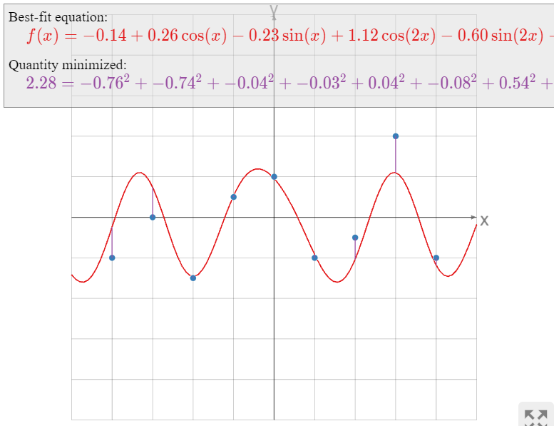
Therefore, the best-fit function is
\[ \begin{split} y \amp\approx -0.1435 + 0.2611\cos(x) -0.2337\sin(x) + 1.116\cos(2x) -0.5997\sin(2x) \\ \amp\qquad\qquad -0.2767\cos(3x) + 0.1076\sin(3x). \end{split} \nonumber \]
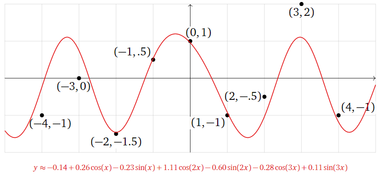
Figure \(\PageIndex{20}\)
As in the previous examples, the best-fit function minimizes the sum of the squares of the vertical distances from the graph of \(y = f(x)\) to the data points.
The next example has a somewhat different flavor from the previous ones.
Find the best-fit ellipse through the points
\[ (0,2),\, (2,1),\, (1,-1),\, (-1,-2),\, (-3,1),\, (-1,-1). \nonumber \]
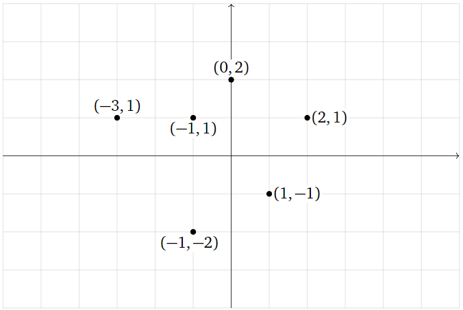
Figure \(\PageIndex{22}\)
What quantity is being minimized?
Solution
The general equation for an ellipse (actually, for a nondegenerate conic section) is
\[ x^2 + By^2 + Cxy + Dx + Ey + F = 0. \nonumber \]
This is an implicit equation: the ellipse is the set of all solutions of the equation, just like the unit circle is the set of solutions of \(x^2+y^2=1.\) To say that our data points lie on the ellipse means that the above equation is satisfied for the given values of \(x\) and \(y\text{:}\)
\[\label{eq:4} \begin{array}{rrrrrrrrrrrrl} (0)^2 &+& B(2)^2 &+& C(0)(2)&+& D(0) &+& E(2)&+& F&=& 0 \\ (2)^2 &+& B(1)^2 &+& C(2)(1)&+& D(2)&+&E(1)&+&F&=& 0 \\ (1)^2&+& B(-1)^2&+&C(1)(-1)&+&D(1)&+&E(-1)&+&F&=&0 \\ (-1)^2&+&B(-2)^2&+&C(-1)(2)&+&D(-1)&+&E(-2)&+&F&=&0 \\ (-3)^2&+&B(1)^2&+&C(-3)(1)&+&D(-3)&+&E(1)&+&F&=&0 \\ (-1)^2&+&B(-1)^2&+&C(-1)(-1)&+&D(-1)&+&E(-1)&+&F&=&0.\end{array}\]
To put this in matrix form, we move the constant terms to the right-hand side of the equals sign; then we can write this as \(Ax=b\) for
\[A=\left(\begin{array}{ccccc}4&0&0&2&1\\1&2&2&1&1\\1&-1&1&-1&1 \\ 4&2&-1&-2&1 \\ 1&-3&-3&1&1 \\ 1&1&-1&-1&1\end{array}\right)\quad x=\left(\begin{array}{c}B\\C\\D\\E\\F\end{array}\right)\quad b=\left(\begin{array}{c}0\\-4\\-1\\-1\\-9\\-1\end{array}\right).\nonumber\]
We compute
\[ A^TA = \left(\begin{array}{ccccc}36&7&-5&0&12 \\ 7&19&9&-5&1 \\ -5&9&16&1&-2 \\ 0&-5&1&12&0 \\ 12&1&-2&0&6\end{array}\right) \qquad A^T b = \left(\begin{array}{c}-19\\17\\20\\-9\\-16\end{array}\right). \nonumber \]
We form an augmented matrix and row reduce:
\[\left(\begin{array}{ccccc|c} 36 &7& -5& 0& 12& -19\\ 7& 19& 9& -5& 1& 17\\ -5& 9& 16& 1& -2& 20\\ 0& -5& 1 &12& 0& -9\\ 12& 1& -2& 0& 6& -16\end{array}\right)\xrightarrow{\text{RREF}}\left(\begin{array}{ccccc|c} 1& 0& 0& 0& 0& 405/266\\ 0& 1& 0& 0& 0& -89/133\\ 0& 0& 1& 0& 0& 201/133\\ 0& 0& 0& 1& 0& -123/266\\ 0& 0& 0& 0& 1& -687/133\end{array}\right).\nonumber\]
The least-squares solution is
\[\hat{x}=\left(\begin{array}{c}405/266\\ -89/133\\ 201/133\\ -123/266\\ -687/133\end{array}\right),\nonumber\]
so the best-fit ellipse is
\[ x^2 + \frac{405}{266} y^2 -\frac{89}{133} xy + \frac{201}{133}x - \frac{123}{266}y - \frac{687}{133} = 0. \nonumber \]
Multiplying through by \(266\text{,}\) we can write this as
\[ 266 x^2 + 405 y^2 - 178 xy + 402 x - 123 y - 1374 = 0. \nonumber \]

Figure \(\PageIndex{23}\)
Now we consider the question of what quantity is minimized by this ellipse. The least-squares solution \(\hat x\) minimizes the sum of the squares of the entries of the vector \(b-A\hat x\text{,}\) or equivalently, of \(A\hat x-b\). The vector \(-b\) contains the constant terms of the left-hand sides of \(\eqref{eq:4}\), and
\[A\hat{x}=\left(\begin{array}{rrrrrrrrr} \frac{405}{266}(2)^2 &-& \frac{89}{133}(0)(2)&+&\frac{201}{133}(0)&-&\frac{123}{266}(2)&-&\frac{687}{133} \\ \frac{405}{266}(1)^2&-& \frac{89}{133}(2)(1)&+&\frac{201}{133}(2)&-&\frac{123}{266}(1)&-&\frac{687}{133} \\ \frac{405}{266}(-1)^2 &-&\frac{89}{133}(1)(-1)&+&\frac{201}{133}(1)&-&\frac{123}{266}(-1)&-&\frac{687}{133} \\ \frac{405}{266}(-2)^2&-&\frac{89}{133}(-1)(-2)&+&\frac{201}{133}(-1)&-&\frac{123}{266}(-2)&-&\frac{687}{133} \\ \frac{405}{266}(1)^2&-&\frac{89}{133}(-3)(1)&+&\frac{201}{133}(-3)&-&\frac{123}{266}(1)&-&\frac{687}{133} \\ \frac{405}{266}(-1)^2&-&\frac{89}{133}(-1)(-1)&+&\frac{201}{133}(-1)&-&\frac{123}{266}(-1)&-&\frac{687}{133}\end{array}\right)\nonumber\]
contains the rest of the terms on the left-hand side of \(\eqref{eq:4}\). Therefore, the entries of \(A\hat x-b\) are the quantities obtained by evaluating the function
\[ f(x,y) = x^2 + \frac{405}{266} y^2 -\frac{89}{133} xy + \frac{201}{133}x - \frac{123}{266}y - \frac{687}{133} \nonumber \]
on the given data points.
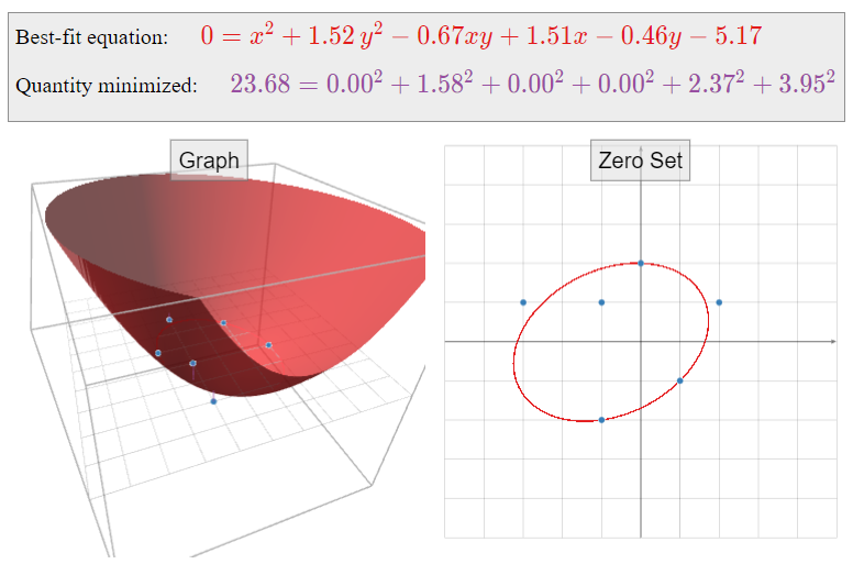
If our data points actually lay on the ellipse defined by \(f(x,y)=0\text{,}\) then evaluating \(f(x,y)\) on our data points would always yield zero, so \(A\hat x-b\) would be the zero vector. This is not the case; instead, \(A\hat x-b\) contains the actual values of \(f(x,y)\) when evaluated on our data points. The quantity being minimized is the sum of the squares of these values:
\[ \begin{split} \amp\text{minimized} = \\ \amp\quad f(0,2)^2 + f(2,1)^2 + f(1,-1)^2 + f(-1,-2)^2 + f(-3,1)^2 + f(-1,-1)^2. \end{split} \nonumber \]
One way to visualize this is as follows. We can put this best-fit problem into the framework of Example \(\PageIndex{8}\) by asking to find an equation of the form
\[ f(x,y) = x^2 + By^2 + Cxy + Dx + Ey + F \nonumber \]
which best approximates the data table
\[ \begin{array}{r|r|c} x & y & f(x,y) \\\hline 0 & 2 & 0 \\ 2 & 1 & 0 \\ 1 & -1 & 0 \\ -1 & -2 & 0 \\ -3 & 1 & 0 \\ -1 & -1 & 0\rlap. \end{array} \nonumber \]
The resulting function minimizes the sum of the squares of the vertical distances from these data points \((0,2,0),\,(2,1,0),\,\ldots\text{,}\) which lie on the \(xy\)-plane, to the graph of \(f(x,y)\).
Gauss invented the method of least squares to find a best-fit ellipse: he correctly predicted the (elliptical) orbit of the asteroid Ceres as it passed behind the sun in 1801.