7.1: A - Números Complejos

\(\usepackage{macros} \newcommand{\lt}{<} \newcommand{\gt}{>} \newcommand{\amp}{&} \)

En este Apéndice damos una breve revisión de las propiedades aritméticas y básicas de los números complejos.

Como motivación, observe que la matriz de rotación

\[ A =\left(\begin{array}{cc}0&-1\\1&0\end{array}\right) \nonumber \]

tiene polinomio característico\(f(\lambda) = \lambda^2 + 1\). Un cero de esta función es una raíz cuadrada de\(-1\). Si queremos que este polinomio tenga una raíz, entonces tenemos que usar un sistema de números más grande: necesitamos declarar por fiat que existe una raíz cuadrada de\(-1\).

Definición\(\PageIndex{1}\): Imaginary Number and Complex Number

1. El número imaginario\(i\) se define para satisfacer la ecuación\(i^2 = -1\).
2. Un número complejo es un número de la forma\(a+bi\text{,}\) donde\(a,b\) están los números reales.

Se denota el conjunto de todos los números complejos\(\mathbb{C}\).

Los números reales son solo los números complejos de la forma\(a + 0i\text{,}\) por lo que\(\mathbb{R}\) está contenida en\(\mathbb{C}\).

Podemos identificarnos\(\mathbb{C}\) con\(\mathbb{R}^2 \) por\(a+bi \longleftrightarrow {a\choose b}\). Entonces cuando dibujamos una imagen de\(\mathbb{C}\text{,}\) dibujamos el plano:

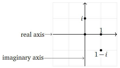
Figura\(\PageIndex{1}\)

Nota\(\PageIndex{1}\): Arithmetic of Complex Numbers

Podemos realizar todas las operaciones aritméticas habituales en números complejos: sumar, restar, multiplicar, dividir, valor absoluto. También hay una nueva operación importante llamada conjugación compleja.

• La adición se realiza por componentes:

  \[ (a + bi) + (c + di) = (a + c) + (b + d)i. \nonumber \]

• La multiplicación se realiza usando distributividad y\(i^2=-1\text{:}\)

  \[ (a+bi)(c+di) = ac + adi + bci + bdi^2 = (ac-bd) + (ad+bc)i. \nonumber \]

• La conjugación compleja reemplaza\(i\) con\(-i\text{,}\) y se denota con una barra:

  \[ \overline{a+bi} = a - bi. \nonumber \]El número\(\overline{a+bi}\) se llama el conjugado complejo de\(a+bi\). Uno comprueba que para cualquiera de dos números complejos\(z,w\text{,}\) tenemos

  \[ \overline{z+w} = \overline{ z} + \overline{ w} \quad\text{and}\quad \overline{zw} = \overline{z}\cdot\overline{w}. \nonumber \]Además, también\((a+bi)(a-bi) = a^2 + b^2\text{,}\) lo\(z\bar z\) es un número real no negativo para cualquier número complejo\(z\).

• El valor absoluto de un número complejo\(z\) es el número real\(|z| = \sqrt{z\overline{ z}}\text{:}\)

  \[ |a+bi| = \sqrt{a^2 + b^2}. \nonumber \]Uno comprueba que\(|zw| = |z|\cdot|w|.\)

• La división por un número real distinto de cero procede por componentes:

  \[ \frac{a+bi}c = \frac ac + \frac bci. \nonumber \]

• La división por un número complejo distinto de cero requiere multiplicar el numerador y el denominador por el conjugado complejo del denominador:

  \[ \frac zw = \frac{z\overline{ w}}{w\overline{ w}} = \frac{z\overline{ w}}{|w|^2}. \nonumber \]Por ejemplo,

  \[ \frac{1+i}{1-i} = \frac{(1+i)^2}{1^2+(-1)^2} = \frac{1+2i+i^2}2 = i. \nonumber \]

• Las partes reales e imaginarias de un número complejo son

  \[ \Re(a+bi) = a \qquad \Im(a+bi) = b. \nonumber \]

El objetivo de introducir números complejos es encontrar raíces de polinomios. Resulta que introducir\(i\) es suficiente para encontrar las raíces de cualquier polinomio.

Teorema\(\PageIndex{1}\): Fundamental Theorem of Algebra

Cada polinomio de grado\(n\) tiene raíces exactamente\(n\) (reales y) complejas, contadas con multiplicidad.

Equivalentemente, si\(f(x) = x^n + a_{n-1}x^{n-1} + \cdots + a_1x + a_0\) es un polinomio de grado\(n\text{,}\) entonces\(f\) factores como

\[ f(x) = (x-\lambda_1)(x-\lambda_2)\cdots(x-\lambda_n) \nonumber \]

para números complejos (no necesariamente distintos)\(\lambda_1,\lambda_2,\ldots,\lambda_n\).

Nota\(\PageIndex{2}\): Degree-2 Polynomials

La fórmula cuadrática da las raíces de un polinomio de grado 2, real o complejo:

\[ f(x) = x^2 + bx + c \implies x = \frac{-b \pm \sqrt{b^2 - 4c}}2. \nonumber \]

Por ejemplo, si\(f(x) = x^2 - \sqrt 2x + 1\text{,}\) entonces

\[ x = \frac{\sqrt 2\pm\sqrt{-2}}2 = \frac{\sqrt 2}2(1\pm i) = \frac{1\pm i}{\sqrt 2}. \nonumber \]

Tenga en cuenta que si\(b,c\) son números reales, entonces las dos raíces son conjugados complejos.

Un número complejo\(z\) es real si y solo si\(z = \bar z\). Esto lleva a la siguiente observación.

Nota \(\PageIndex{3}\)

Si\(f\) es un polinomio con coeficientes reales, y si\(\lambda\) es una raíz compleja de\(f\text{,}\) entonces así es\(\overline{\lambda}\text{:}\)

\[\begin{aligned}0=\overline{f(\lambda )}&=\overline{\lambda^n+a_{n-1}\lambda^{n-1}+\cdots +a_1\lambda +a_0} \\ &=\overline{\lambda}^n+a_{n-1}\overline{\lambda}^{n-1}+\cdots +a_1\overline{\lambda}+a_0=f(\overline{\lambda}).\end{aligned}\]

Por lo tanto, las raíces complejas de polinomios reales vienen en pares conjugados.

Nota\(\PageIndex{4}\): Degree-3 Polynomials

Un polinomio cúbico real tiene tres raíces reales, o una raíz real y un par conjugado de raíces complejas.

Por ejemplo,\(f(x) = x^3-x = x(x-1)(x+1)\) tiene tres raíces reales; su gráfica se ve así:

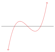
Figura\(\PageIndex{2}\)

Por otro lado, el polinomio

\[ g(x) = x^3-5x^2+x-5 = (x-5)(x^2+1) = (x-5)(x+i)(x-i) \nonumber \]

tiene una raíz real\(5\) y un par conjugado de raíces complejas\(\pm i\). Su gráfica se ve así:

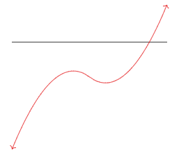
Figura\(\PageIndex{3}\)