2.3: Visualización de Aritmética Matricial en 2D

Última actualización
Guardar como PDF

Page ID: 116406

$ \newcommand{\vecs}[1]{\overset { \scriptstyle \rightharpoonup} {\mathbf{#1}} } $ $ \newcommand{\vecd}[1]{\overset{-\!-\!\rightharpoonup}{\vphantom{a}\smash {#1}}} $$\newcommand{\id}{\mathrm{id}}$ $ \newcommand{\Span}{\mathrm{span}}$ $ \newcommand{\kernel}{\mathrm{null}\,}$ $ \newcommand{\range}{\mathrm{range}\,}$ $ \newcommand{\RealPart}{\mathrm{Re}}$ $ \newcommand{\ImaginaryPart}{\mathrm{Im}}$ $ \newcommand{\Argument}{\mathrm{Arg}}$ $ \newcommand{\norm}[1]{\| #1 \|}$ $ \newcommand{\inner}[2]{\langle #1, #2 \rangle}$ $ \newcommand{\Span}{\mathrm{span}}$ $\newcommand{\id}{\mathrm{id}}$ $ \newcommand{\Span}{\mathrm{span}}$ $ \newcommand{\kernel}{\mathrm{null}\,}$ $ \newcommand{\range}{\mathrm{range}\,}$ $ \newcommand{\RealPart}{\mathrm{Re}}$ $ \newcommand{\ImaginaryPart}{\mathrm{Im}}$ $ \newcommand{\Argument}{\mathrm{Arg}}$ $ \newcommand{\norm}[1]{\| #1 \|}$ $ \newcommand{\inner}[2]{\langle #1, #2 \rangle}$ $ \newcommand{\Span}{\mathrm{span}}$$\newcommand{\AA}{\unicode[.8,0]{x212B}}$

Objetivos de aprendizaje

T/F: Dos vectores con la misma longitud y dirección son iguales aunque comiencen desde diferentes lugares.
¿Se puede visualizar la adición de vectores usando qué ley?
T/F: Multiplicar un vector por 2 duplica su longitud.
¿Qué hacen los matemáticos?
T/F: Multiplicar un vector por una matriz siempre cambia su longitud y dirección.

Cuando aprendimos por primera vez a sumar números, fue útil fotografiar una línea numérica:$2+3=5$ podría ser fotografiada comenzando en 0, saliendo 2 marcas de garrapatas, luego otras 3, y luego dándonos cuenta de que movimos 5 marcas de 0. Visualizaciones similares nos ayudaron a entender qué$2-3$ significaba y qué$2\times 3$ significaba.

Ahora investigamos una forma de imaginar la aritmética matricial, en particular, las operaciones que involucran vectores de columna. Esto no sólo nos ayudará a entender mejor las operaciones aritméticas, sino que abrirá la puerta a una gran riqueza de estudio interesante. Visualizar la aritmética matricial tiene una amplia variedad de aplicaciones, siendo las más comunes las gráficas por computadora. Si bien a menudo pensamos en estos gráficos en términos de videojuegos, existen otras numerosas aplicaciones importantes. Por ejemplo, los químicos y biólogos suelen utilizar modelos informáticos para “visualizar” moléculas complejas para “ver” cómo interactúan con otras moléculas.

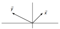
Comenzaremos con vectores en dos dimensiones (2D) —es decir, vectores con sólo dos entradas. Suponemos que el lector está familiarizado con el plano cartesiano, es decir, trazar puntos y graficar funciones en “el$y$ plano$x$ —”. Gráficamos vectores de una manera muy similar a los puntos de trazado. Dado el vector\[\vec{x}=\left[\begin{array}{c}{1}&{2}\end{array}\right] , \nonumber \] dibujamos$\vec{x}$ dibujando una flecha cuya punta es 1 unidad a la derecha y 2 unidades hacia arriba desde su origen. $^{1}$

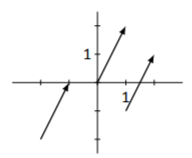
$clipboard_ee100fecf16758ba73c9bc5e1df4f16c9.png$

Figura$\PageIndex{1}$: Diversos dibujos de$\vec{x}$

Al dibujar vectores, no especificamos dónde comienzas a dibujar; todo lo que especificamos es dónde se encuentra la punta en función de dónde empezamos. La figura$\PageIndex{1}$ muestra el vector$\vec{x}$ dibujado de 3 vías. De alguna manera, la forma “más común” de dibujar un vector tiene el inicio de la flecha en el origen, pero esta no es de ninguna manera la única forma de dibujar el vector.

Practicemos este concepto dibujando varios vectores a partir de puntos de partida dados.

Ejemplo$\PageIndex{1}$

Let

\[\vec{x}=\left[\begin{array}{c}{1}\\{-1}\end{array}\right]\quad\vec{y}=\left[\begin{array}{c}{2}\\{3}\end{array}\right]\quad\text{and}\quad\vec{z}=\left[\begin{array}{c}{-3}\\{2}\end{array}\right] . \nonumber \]

Dibuja a$\vec{x}$ partir del punto$(0, −1)$; dibujar a$\vec{y}$ partir del punto$(−1, −1)$, y dibujar a$\vec{z}$ partir del punto$(2, −1)$.

Solución

Para dibujar$\vec{x}$, comienza en el punto$(0,-1)$ como se indica, luego mueve hacia la derecha una unidad y baja una unidad y dibuja la punta. Así la flecha “apunta” de$(0,-1)$ a$(1,-2)$.

Para dibujar$\vec{y}$, se nos dice que comencemos y el punto$(-1,-1)$. Dibujamos la punta moviéndonos hacia la derecha 2 unidades y subiendo 3 unidades; de ahí$\vec{y}$ apunta de$(-1,-1)$ a (1,2).

Para dibujar$\vec{z}$, partimos en$(2,-1)$ y dibujamos la punta 3 unidades a la izquierda y 2 unidades hacia arriba;$\vec{z}$ puntos de$(2,-1)$ a$(-1,1)$.

Cada vector se dibuja como se muestra en la Figura$\PageIndex{2}$.

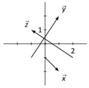
$clipboard_e7a44062393d3b40d4a18c77636bf4f4d.png$

Figura$\PageIndex{2}$: Dibujo de vectores$\vec{x}$,$\vec{y}$ y$\vec{z}$ en Ejemplo$\PageIndex{1}$

¿Cómo se dibuja el vector cero,$\vec{0}=\left[\begin{array}{c}{0}\\{0}\end{array}\right]$? $^{2}$Siguiendo nuestro procedimiento básico, comenzamos por ir 0 unidades en la$x$ dirección, seguido de 0 unidades en la$y$ dirección. En otras palabras, no vamos a ningún lado. En general, en realidad no dibujamos$\vec{0}$. En el mejor de los casos, se puede dibujar un círculo oscuro en el origen para transmitir la idea de que$\vec{0}$, al comenzar por el origen, apunta al origen.

En la Sección 2.1 aprendimos sobre las operaciones aritméticas matriciales: suma matricial y multiplicación escalar. Investiguemos cómo podemos “dibujar” estas operaciones.

Adición de vectores

Dados dos vectores$\vec{x}$ y$\vec{y}$, ¿cómo dibujamos el vector$\vec{x}+\vec{y}$? Veamos esto en el contexto de un ejemplo, luego estudiemos el resultado.

Ejemplo$\PageIndex{2}$

Let

\[\vec{x}=\left[\begin{array}{c}{1}\\{1}\end{array}\right]\quad\text{and}\quad\vec{y}=\left[\begin{array}{c}{3}\\{1}\end{array}\right] .\nonumber \]

Sketch$\vec{x}$,$\vec{y}$ y$\vec{x}+\vec{y}$.

Solución

No se dio un punto de partida para dibujar cada vector; por defecto, comenzaremos en el origen. (Esto es en muchos sentidos agradable; esto significa que el vector$\left[\begin{array}{c}{3}\\{1}\end{array}\right]$ “apunta” al punto (3,1).) Primero computamos$\vec{x}+\vec{y}$:

\[\vec{x}+\vec{y}=\left[\begin{array}{c}{1}\\{1}\end{array}\right]+\left[\begin{array}{c}{3}\\{1}\end{array}\right]=\left[\begin{array}{c}{4}\\{2}\end{array}\right] \nonumber \]

El bosquejar cada uno da la imagen en la Figura$\PageIndex{3}$.

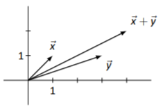
$clipboard_eaa48f2b609ccd2c2adbee8c045e6f55d.png$

Figura$\PageIndex{3}$: Adición de vectores$\vec{x}$ y$\vec{y}$ en Ejemplo$\PageIndex{2}$

Este ejemplo es bastante básico; nos dieron dos vectores, nos dijeron que los agregáramos juntos, luego bosquejemos los tres vectores. Nuestro trabajo ahora es volver atrás y tratar de ver una relación entre los dibujos de$\vec{x}$,$\vec{y}$ y$\vec{x}+\vec{y}$. ¿Ves alguna?

Aquí hay una forma de interpretar la adición de$\vec{x}$ a$\vec{y}$. Independientemente de donde empecemos, dibujamos$\vec{x}$. Ahora, desde la punta de$\vec{x}$, dibuja$\vec{y}$. El vector$\vec{x}+\vec{y}$ es el vector que se encuentra dibujando una flecha desde el origen de$\vec{x}$ hasta la punta de$\vec{y}$. De igual manera, podríamos comenzar por dibujar$\vec{y}$. Entonces, a partir de la punta de$\vec{y}$, podemos dibujar$\vec{x}$. Finalmente, dibuja$\vec{x}+\vec{y}$ dibujando el vector que comienza en el origen de$\vec{y}$ y termina en la punta de$\vec{x}$.

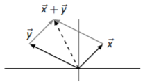
La imagen de la Figura$\PageIndex{4}$ ilustra esto. Los vectores grises demuestran dibujar el segundo vector desde la punta del primero; dibujamos el vector$\vec{x}+\vec{y}$ discontinuas para diferenciarlo del resto. También llenamos ligeramente el paralelogramo cuyos lados opuestos son los vectores$\vec{x}$ y$\vec{y}$. Esto resalta lo que se conoce como la Ley del Paralelogramo.

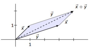
$clipboard_e1d1958604149a8b3fc8d549f92ff05c8.png$

Figura$\PageIndex{4}$: Agregar vectores gráficamente usando la Ley de Paralelogramo

Idea Clave$\PageIndex{1}$: Parallelogram Law

Para dibujar el vector$\vec{x}+\vec{y}$, se puede dibujar el paralelogramo con$\vec{x}$ y$\vec{y}$ como sus lados. El vector que apunta desde el vértice donde$\vec{x}$ y$\vec{y}$ se originan al vértice donde$\vec{x}$ y se$\vec{y}$ encuentran es el vector$\vec{x}+\vec{y}$.

Conocer todo esto nos permite dibujar la suma de dos vectores sin saber específicamente cuáles son los vectores, como demostramos en el siguiente ejemplo.

Ejemplo$\PageIndex{3}$

Considera los vectores$\vec{x}$ y$\vec{y}$ como se dibuja en la Figura$\PageIndex{5}$. Esbozar el vector$\vec{x}+\vec{y}$.

Solución

$clipboard_eecd6ef94e3229eb963199bd77fa56be5.png$

Figura$\PageIndex{5}$: Vectores$\vec{x}$ y$\vec{y}$ en Ejemplo$\PageIndex{3}$

Aplicaremos la Ley de Paralelogramo, tal como se da en Idea Clave$\PageIndex{1}$. Como antes, dibujamos$\vec{x}+\vec{y}$ discontinuo para diferenciarlo. El resultado se da en la Figura$\PageIndex{6}$.

$clipboard_e7b4dce14ca15d1093ba86c0a43eae6fa.png$

Figura$\PageIndex{6}$: Vectores$\vec{x}$,$\vec{y}$ y$\vec{x}+\vec{y}$ en Ejemplo$\PageIndex{3}$

Multiplicación escalar

Después de aprender sobre la adición matricial, aprendimos sobre la multiplicación escalar. Aplicamos ese concepto ahora a los vectores y vemos cómo se representa gráficamente este concepto.

Ejemplo$\PageIndex{4}$

Let

\[\vec{x}=\left[\begin{array}{c}{1}\\{1}\end{array}\right]\quad\text{and}\quad\vec{y}=\left[\begin{array}{c}{-2}\\{1}\end{array}\right] .\nonumber \]

Bosquejo$\vec{x}$$\vec{y}$,,$3\vec{x}$ y$-1\vec{y}$.

Solución

Comenzamos por la computación$3\vec{x}$ y$-\vec{y}$:

\[3\vec{x}=\left[\begin{array}{c}{3}\\{3}\end{array}\right]\quad\text{and}\quad -\vec{y}=\left[\begin{array}{c}{2}\\{-1}\end{array}\right] . \nonumber \]

Los cuatro vectores se esbozan en la Figura$\PageIndex{7}$.

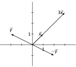
$clipboard_ee689746c7ebfd8b7f9d3300efe7fa60b.png$

Figura$\PageIndex{7}$: Vectores$\vec{x}$,$\vec{y}$,$3\vec{x}$ y$-\vec{y}$ en Ejemplo$\PageIndex{4}$

Como solemos hacer, veamos el ejemplo anterior y veamos qué podemos aprender de él. Eso podemos ver$\vec{x}$ y$3\vec{x}$ apuntar en la misma dirección (se encuentran en la misma línea), pero sólo$3\vec{x}$ es más largo que$\vec{x}$. (De hecho, parece que$3\vec{x}$ es 3 veces más largo que$\vec{x}$. ¿Lo es? ¿Cómo medimos la longitud?)

También vemos eso$\vec{y}$ y$-\vec{y}$ parece que tienen la misma longitud y se encuentran en la misma línea, pero apuntan en sentido contrario.

Un vector transmite inherentemente dos piezas de información: longitud y dirección. Multiplicar un vector por un escalar positivo$c$ estira los vectores por un factor de$c$; multiplicando por un escalar negativo$c$ ambos estira el vector y lo hace apuntar en la dirección opuesta.

Sabiendo esto, podemos bosquejar múltiplos escalares de vectores sin saber específicamente cuáles son, como lo hacemos en el siguiente ejemplo.

Ejemplo$\PageIndex{5}$

Dejar vectores$\vec{x}$ y$\vec{y}$ ser como en la Figura$\PageIndex{8}$. Dibujar$3\vec{x}$,$-2\vec{x}$, y$\frac{1}{2}\vec{y}$.

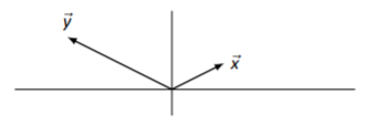
$clipboard_e671e2f1985e077c7850ede98bc227fa5.png$

Figura$\PageIndex{8}$: Vectores$\vec{x}$ y$\vec{y}$ en Ejemplo$\PageIndex{5}$

Solución

Para dibujar$3\vec{x}$, dibujamos un vector en la misma dirección que$\vec{x}$, pero 3 veces más largo. Para dibujar$-2\vec{x}$, dibujamos un vector el doble de largo que$\vec{x}$ en la dirección opuesta; para dibujar$\frac{1}{2}\vec{y}$, dibujamos un vector de la mitad de la longitud de$\vec{y}$ en la misma dirección que$\vec{y}$. Nuevamente usamos el valor por defecto de dibujar todos los vectores comenzando en el origen. Todo esto se muestra en la Figura$\PageIndex{9}$.

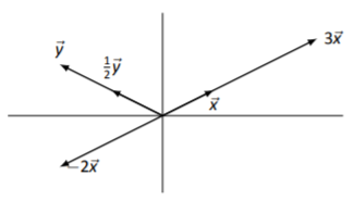
$clipboard_e730529999cba3617d3761532bb74eb57.png$

Figura$\PageIndex{9}$: Vectores$\vec{x}$,$\vec{y}$,$3\vec{x}$,$-2x$ y$\frac{1}{2}\vec{x}$ en Ejemplo$\PageIndex{5}$

Resta vectorial

La operación básica final a considerar entre dos vectores es la de sustracción vectorial: vectores dados$\vec{x}$ y$\vec{y}$, ¿cómo dibujamos$\vec{x}-\vec{y}$?

Si sabemos explícitamente qué$\vec{x}$ y$\vec{y}$ son, simplemente podemos calcular lo que$\vec{x}-\vec{y}$ es y luego dibujarlo. También podemos pensar en términos de adición de vectores y multiplicación escalar: podemos agregar los vectores$\vec{x}+(-1)\vec{y}$. Es decir, podemos dibujar$\vec{x}$ y dibujar$-\vec{y}$, luego agregarlos como hicimos en Ejemplo$\PageIndex{3}$. Esto es especialmente útil no sabemos explícitamente qué$\vec{x}$ y$\vec{y}$ somos.

Ejemplo$\PageIndex{6}$

Dejar vectores$\vec{x}$ y$\vec{y}$ ser como en la Figura$\PageIndex{10}$. Empate$\vec{x}-\vec{y}$.

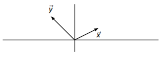
$clipboard_e81e1a72da6e0dc89897978821f386525.png$

Figura$\PageIndex{10}$: Vectores$\vec{x}$ y$\vec{y}$ en Ejemplo$\PageIndex{6}$

Solución

Para dibujar$\vec{x}-\vec{y}$, primero dibujaremos$-\vec{y}$ y luego aplicaremos la Ley de Paralelogramo para agregar$\vec{x}$ a$-\vec{y}$. Ver Figura$\PageIndex{11}$.

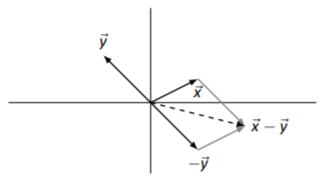
$clipboard_ee0a10fa6ce0a35c744ddeabb6e21b383.png$

Figura$\PageIndex{11}$: Vectores$\vec{x}$,$\vec{y}$ y$\vec{x}-\vec{y}$ en Ejemplo$\PageIndex{6}$

En Figura$\PageIndex{12}$, redibujamos Figura$\PageIndex{11}$ de Ejemplo$\PageIndex{6}$ pero eliminamos los vectores grises que tienden a agregar desorden, y redibujamos el vector$\vec{x}-\vec{y}$ punteado para que comience desde la punta de$\vec{y}$. $^{3}$Tenga en cuenta que la versión punteada de$\vec{x}-\vec{y}$ puntos de$\vec{y}$ a$\vec{x}$. Este es un “atajo” para dibujar$\vec{x}-\vec{y}$; simplemente dibuja el vector que comienza en la punta de$\vec{y}$ y termina en la punta de$\vec{x}$. Esto es importante así que lo hacemos una Idea Clave.

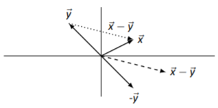
$clipboard_eb6e3c041c8055326108469c2a282accb.png$

Figura$\PageIndex{12}$: Redibujar vector$\vec{x}-\vec{y}$

Idea Clave$\PageIndex{2}$: Vector Subtraction

Para dibujar el vector$\vec{x}-\vec{y}$, dibujar$\vec{x}$ y$\vec{y}$ para que tengan el mismo origen. El vector$\vec{x}-\vec{y}$ es el vector que comienza desde la punta de$\vec{y}$ y apunta a la punta de$\vec{x}$.

Practicemos esto una vez más con un ejemplo rápido.

Ejemplo$\PageIndex{7}$

Dejar$\vec{x}$ y$\vec{y}$ ser como en la Figura$\PageIndex{13}$ (a), Dibujar$\vec{x}-\vec{y}$.

Solución

Simplemente aplicamos Key Idea$\PageIndex{2}$: dibujamos una flecha de$\vec{y}$ a$\vec{x}$. Lo hacemos en Figura$\PageIndex{13}$;$\vec{x}-\vec{y}$ es discontinuo.

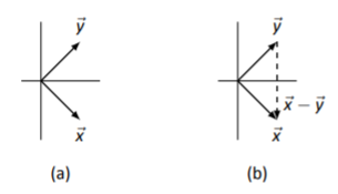
$clipboard_ebc48839c92cf534a3760eb2cbc44349d.png$

Figura$\PageIndex{13}$: Vectores$\vec{x}$,$\vec{y}$ y$\vec{x}-\vec{y}$ en Ejemplo$\PageIndex{7}$

Longitud del vector

Cuando discutimos la multiplicación escalar, hicimos referencia a una pregunta fundamental: ¿Cómo medimos la longitud de un vector? La geometría básica nos da una respuesta en el caso bidimensional que estamos tratando ahora mismo, y posteriormente podremos extender estas ideas a dimensiones superiores.

Considera Figura$\PageIndex{14}$. $\vec{x}$Se dibuja un vector en negro, y se han dibujado líneas discontinuas y punteadas para convertirlo en la hipotenusa de un triángulo rectángulo.

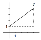
$clipboard_e1999d0fbf0f93189bbe3c82df0fbe01f.png$

Figura$\PageIndex{14}$: Medición de la longitud de un vector

Es fácil ver que la línea discontinua tiene longitud 4 y la línea punteada tiene longitud 3. Vamos a dejar$c$ denotar la longitud de$\vec{x}$; según el Teorema de Pitágoras,$4^2+3^2 = c^2$. Así$c^2 = 25$ y rápidamente deducimos eso$c=5$.

Observe que en nuestra figura,$\vec{x}$ va a la derecha 4 unidades y luego arriba 3 unidades. En otras palabras, podemos escribir\[\vec{x}=\left[\begin{array}{c}{4}\\{3}\end{array}\right] . \nonumber \] Aprendimos arriba que la longitud de$\vec{x}$ es$\sqrt{4^2+3^2}$. $^{4}$Esto sugiere un cálculo básico que funciona para todos los vectores$\vec{x}$, y definimos la longitud de un vector de acuerdo con esta regla.

Definición: Longitud del vector

Let

\[\vec{x}=\left[\begin{array}{c}{x_{1}}\\{x_{2}}\end{array}\right] . \nonumber \]

La longitud de$\vec{x}$, denota$||\vec{x}||$, es

\[||\vec{x}||=\sqrt{x_{1}^{2}+x_{2}^{2}} . \nonumber \]

Ejemplo$\PageIndex{8}$

Encuentra la longitud de cada uno de los vectores que se indican a continuación.

\[\vec{x}_{1}=\left[\begin{array}{c}{1}\\{1}\end{array}\right]\quad\vec{x}_{2}=\left[\begin{array}{c}{2}\\{-3}\end{array}\right]\quad\vec{x}_{3}=\left[\begin{array}{c}{.6}\\{.8}\end{array}\right]\quad\vec{x}_{4}=\left[\begin{array}{c}{3}\\{0}\end{array}\right]\nonumber \]

Solución

Aplicamos Longitud del Vector de Definición a cada vector.
\[\begin{aligned} ||\vec{x}_{1}|| &= \sqrt{1^2+1^2} = \sqrt{2}.\\ ||\vec{x}_{2}|| &= \sqrt{2^2+(-3)^2} = \sqrt{13}.\\ ||\vec{x}_{3}|| &= \sqrt{.6^2 +.8^2} = \sqrt{.36+.64} = 1.\\ ||\vec{x}_{4}|| &= \sqrt{3^2+0} = 3.\end{aligned} \nonumber \]

Ahora que sabemos cómo calcular la longitud de un vector, volvamos a visitar una declaración que hicimos mientras exploramos Ejemplos$\PageIndex{4}$ and $\PageIndex{5}$: “Multiplying a vector by a positive scalar $c$ stretches the vectors by a factor of $c$ $\ldots$” At that time, we did not know how to measure the length of a vector, so our statement was unfounded. In the following example, we will confirm the truth of our previous statement.

Example $\PageIndex{9}$

Let $\vec{x}=\left[\begin{array}{c}{2}\\{-1}\end{array}\right]$. Compute $||\vec{x}||$, $||3\vec{x}||$, $||-2\vec{x}||$, and $||c\vec{x}||$, where $c$ is a scalar.

Solution

We apply Definition Vector Length to each of the vectors.

$||\vec{x}|| = \sqrt{4+1} = \sqrt{5}$.

Before computing the length of $||3\vec{x}||$, we note that $3\vec{x} = \left[\begin{array}{c}{6}\\{-3}\end{array}\right]$.

$||3\vec{x}|| = \sqrt{36+9} = \sqrt{45} = 3\sqrt{5} = 3||\vec{x}||.$

Before computing the length of $||-2\vec{x}||$, we note that $-2\vec{x} = \left[\begin{array}{c}{-4}\\{2}\end{array}\right]$.

$||-2\vec{x}|| = \sqrt{16+4} = \sqrt{20} = 2\sqrt{5} = 2||\vec{x}||.$

Finally, to compute $||c\vec{x}||$, we note that $c\vec{x} = \left[\begin{array}{c}{2c}\\{-c}\end{array}\right]$. Thus:

$||c\vec{x}|| = \sqrt{(2c)^2 + (-c)^2} = \sqrt{4c^2 + c^2} = \sqrt{5c^2} = |c|\sqrt{5}.$

This last line is true because the square root of any number squared is the absolute value of that number (for example, $\sqrt{(-3)^2} = 3$).

The last computation of our example is the most important one. It shows that, in general, multiplying a vector $\vec{x}$ by a scalar $c$ stretches $\vec{x}$ by a factor of $|c|$ (and the direction will change if $c$ is negative). This is important so we’ll make it a Theorem.

Theorem $\PageIndex{1}$

Vector Length and Scalar Multiplication

Let $\vec{x}$ be a vector and let c be a scalar. Then the length of $c\vec{x}$ is

\[||c\vec{x}||=|c|\cdot ||\vec{x}|| . \nonumber \]

Matrix - Vector Multiplication

The last arithmetic operation to consider visualizing is matrix multiplication. Specifically, we want to visualize the result of multiplying a vector by a matrix. In order to multiply a 2D vector by a matrix and get a 2D vector back, our matrix must be a square, $2\times 2$ matrix.$^{5}$

We’ll start with an example. Given a matrix $A$ and several vectors, we’ll graph the vectors before and after they’ve been multiplied by $A$ and see what we learn.

Example $\PageIndex{10}$

Let $A$ be a matrix, and $\vec{x}$, $\vec{y}$, and $\vec{z}$ be vectors as given below.

\[A=\left[\begin{array}{cc}{1}&{4}\\{2}&{3}\end{array}\right],\quad\vec{x}=\left[\begin{array}{c}{1}\\{1}\end{array}\right],\quad\vec{y}=\left[\begin{array}{c}{-1}\\{1}\end{array}\right],\quad\vec{z}=\left[\begin{array}{c}{3}\\{-1}\end{array}\right]\nonumber \]

Graph $\vec{x}$, $\vec{y}$ and $\vec{z}$, as well as $A\vec{x}$, $A\vec{y}$ and $A\vec{z}$.

Solution

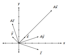
$clipboard_edcd187efdc2ea575c48d86b38613cd05.png$

Figure $\PageIndex{15}$: Multiplying vectors by a matrix in Example $\PageIndex{10}$.

It is straightforward to compute:

\[A\vec{x}=\left[\begin{array}{c}{5}\\{5}\end{array}\right],\quad A\vec{y}=\left[\begin{array}{c}{3}\\{1}\end{array}\right],\quad\text{and}\quad A\vec{z}=\left[\begin{array}{c}{-1}\\{3}\end{array}\right]. \nonumber \]

The vectors are sketched in Figure $\PageIndex{15}$.

There are several things to notice. When each vector is multiplied by $A$, the result is a vector with a different length (in this example, always longer), and in two of the cases (for $\vec{y}$ and $\vec{z}$), the resulting vector points in a different direction.

This isn’t surprising. In the previous section we learned about matrix multiplication, which is a strange and seemingly unpredictable operation. Would you expect to see some sort of immediately recognizable pattern appear from multiplying a matrix and a vector?$^{6}$ In fact, the surprising thing from the example is that $\vec{x}$ and $A\vec{x}$ point in the same direction! Why does the direction of $\vec{x}$ not change after multiplication by $A$? (We’ll answer this in Section 4.1 when we learn about something called “eigenvectors.”)

Different matrices act on vectors in different ways.$^{7}$ Some always increase the length of a vector through multiplication, others always decrease the length, others increase the length of some vectors and decrease the length of others, and others still don’t change the length at all. A similar statement can be made about how matrices affect the direction of vectors through multiplication: some change every vector’s direction, some change “most” vector’s direction but leave some the same, and others still don’t change the direction of any vector.

How do we set about studying how matrix multiplication affects vectors? We could just create lots of different matrices and lots of different vectors, multiply, then graph, but this would be a lot of work with very little useful result. It would be too hard to find a pattern of behavior in this.$^{8}$

Instead, we’ll begin by using a technique we’ve employed often in the past. We have a “new” operation; let’s explore how it behaves with “old” operations. Specifically, we know how to sketch vector addition. What happens when we throw matrix multiplication into the mix? Let’s try an example.

Example $\PageIndex{11}$

Let $A$ be a matrix and $\vec{x}$ and $\vec{y}$ be vectors as given below.

\[A=\left[\begin{array}{cc}{1}&{1}\\{1}&{2}\end{array}\right],\quad\vec{x}=\left[\begin{array}{c}{2}\\{1}\end{array}\right],\quad\vec{y}=\left[\begin{array}{c}{-1}\\{1}\end{array}\right]\nonumber \]

Sketch $\vec{x}+\vec{y}$, $A\vec{x}$, $A\vec{y}$, and $A(\vec{x}+\vec{y})$.

Solution

It is pretty straightforward to compute:

\[\vec{x}+\vec{y}=\left[\begin{array}{c}{1}\\{2}\end{array}\right];\quad A\vec{x}=\left[\begin{array}{c}{3}\\{4}\end{array}\right];\quad A\vec{y}=\left[\begin{array}{c}{0}\\{1}\end{array}\right],\quad A(\vec{x}+\vec{y})=\left[\begin{array}{c}{3}\\{5}\end{array}\right] . \nonumber \]

In Figure $\PageIndex{16}$, we have graphed the above vectors and have included dashed gray vectors to highlight the additive nature of $\vec{x}+\vec{y}$ and $A(\vec{x}+\vec{y})$. Does anything strike you as interesting?

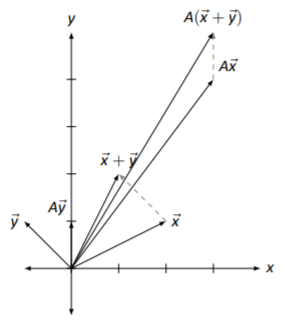
$clipboard_e0bbd180cf319fa467f04b9d9aca53979.png$

Figure $\PageIndex{16}$: Vector addition and matrix multiplication in Example $\PageIndex{11}$.

Let’s not focus on things which don’t matter right now: let’s not focus on how long certain vectors became, nor necessarily how their direction changed. Rather, think about how matrix multiplication interacted with the vector addition.

In some sense, we started with three vectors, $\vec{x}$, $\vec{y}$, and $\vec{x}+\vec{y}$. This last vector is special; it is the sum of the previous two. Now, multiply all three by $A$. What happens? We get three new vectors, but the significant thing is this: the last vector is still the sum of the previous two! (We emphasize this by drawing dotted vectors to represent part of the Parallelogram Law.)

Of course, we knew this already: we already knew that $A\vec{x}+A\vec{y}=A(\vec{x}+\vec{y})$, for this is just the Distributive Property. However, now we get to see this graphically.

In Section 5.1 we’ll study in greater depth how matrix multiplication affects vectors and the whole Cartesian plane. For now, we’ll settle for simple practice: given a matrix and some vectors, we’ll multiply and graph. Let’s do one more example.

Example $\PageIndex{12}$

Let $A$, $\vec{x}$, $\vec{y}$, and $\vec{z}$ be as given below.

\[A=\left[\begin{array}{cc}{1}&{-1}\\{1}&{-1}\end{array}\right],\quad\vec{x}=\left[\begin{array}{c}{1}\\{1}\end{array}\right],\quad\vec{y}=\left[\begin{array}{c}{-1}\\{1}\end{array}\right],\quad\vec{z}=\left[\begin{array}{c}{4}\\{1}\end{array}\right]\nonumber \]

Graph $\vec{x}$, $\vec{y}$ and $\vec{z}$, as well as $A\vec{x}$, $A\vec{y}$ and $A\vec{z}$.

Solution

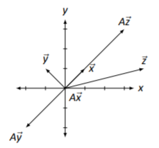
$clipboard_e205ba013b99c89c384286243e16512cd.png$

Figure $\PageIndex{17}$: Multiplying vectors by a matrix in Example $\PageIndex{12}$.

It is straightforward to compute: \[A\vec{x}=\left[\begin{array}{c}{0}\\{0}\end{array}\right],\quad A\vec{y}=\left[\begin{array}{c}{-2}\\{-2}\end{array}\right],\quad\text{and}\quad A\vec{z}=\left[\begin{array}{c}{3}\\{3}\end{array}\right]. \nonumber \] The vectors are sketched in Figure $\PageIndex{17}$.

These results are interesting. While we won’t explore them in great detail here, notice how $\vec{x}$ got sent to the zero vector. Notice also that $A\vec{x}$, $A\vec{y}$ and $A\vec{z}$ are all in a line (as well as $\vec{x}$!). Why is that? Are $\vec{x}$, $\vec{y}$ and $\vec{z}$ just special vectors, or would any other vector get sent to the same line when multiplied by ?$^{9}$

This section has focused on vectors in two dimensions. Later on in this book, we’ll extend these ideas into three dimensions (3D).

In the next section we’ll take a new idea (matrix multiplication) and apply it to an old idea (solving systems of linear equations). This will allow us to view an old idea in a new way – and we’ll even get to “visualize” it.

Footnotes

[1] To help reduce clutter, in all figures each tick mark represents one unit.

[2] Vectors are just special types of matrices. The zero vector, $\vec{0}$, is a special type of zero matrix, $\mathbf{0}$. It helps to distinguish the two by using different notation.

[3] Remember that we can draw vectors starting from anywhere.

[4] Remember that $\sqrt{4^2+3^2} \neq 4+3$!

[5] We can multiply a $3\times 2$ matrix by a 2D vector and get a 3D vector back, and this gives very interesting results. See Section 5.2.

[6] This is a rhetorical question; the expected answer is “No.”

[7] That’s one reason we call them “different.”

[8] Remember, that’s what mathematicians do. We look for patterns.

[9] Don’t just sit there, try it out!

Search

Ejemplo\(\PageIndex{2}\)

Idea Clave\(\PageIndex{1}\): Parallelogram Law

Ejemplo\(\PageIndex{3}\)

Ejemplo\(\PageIndex{4}\)

Ejemplo\(\PageIndex{5}\)

Ejemplo\(\PageIndex{6}\)

Idea Clave\(\PageIndex{2}\): Vector Subtraction

Ejemplo\(\PageIndex{7}\)

Definición: Longitud del vector

Ejemplo\(\PageIndex{8}\)

Example \(\PageIndex{9}\)

Theorem \(\PageIndex{1}\)

Example \(\PageIndex{10}\)

Example \(\PageIndex{11}\)

Example \(\PageIndex{12}\)

Objetivos de aprendizaje

Ejemplo\(\PageIndex{1}\)

Adición de vectores

Ejemplo\(\PageIndex{2}\)

Idea Clave\(\PageIndex{1}\): Parallelogram Law

Ejemplo\(\PageIndex{3}\)

Multiplicación escalar

Ejemplo\(\PageIndex{4}\)

Ejemplo\(\PageIndex{5}\)

Resta vectorial

Ejemplo\(\PageIndex{6}\)

Idea Clave\(\PageIndex{2}\): Vector Subtraction

Ejemplo\(\PageIndex{7}\)

Longitud del vector

Definición: Longitud del vector

Ejemplo\(\PageIndex{8}\)

Example \(\PageIndex{9}\)

Theorem \(\PageIndex{1}\)

Matrix - Vector Multiplication

Example \(\PageIndex{10}\)

Example \(\PageIndex{11}\)

Example \(\PageIndex{12}\)

Footnotes