6.4: Discontinuidades de Derivados

Teorema\(\PageIndex{1}\): Intermediate Value Theorem for Derivatives

Supongamos que\(f\) es diferenciable en un intervalo abierto\(I, a, b \in I,\)\(\lambda \in \mathbb{R}\) y\(a<b .\) Si y cualquiera\(f^{\prime}(a)<\lambda<f^{\prime}(b)\) o\(f^{\prime}(a)>\lambda>f^{\prime}(b),\) entonces existe\(c \in(a, b)\) tal que\(f^{\prime}(c)=\lambda\).

Prueba

Supongamos\(f^{\prime}(a)<\lambda<f^{\prime}(b)\) y definimos\(g: I \rightarrow \mathbb{R}\) por\(g(x)=f(x)-\lambda x\). Entonces\(g\) es diferenciable encendido\(I,\) y así continuo en\([a, b] .\) Let\(c\) ser un punto\([a, b]\) en el que\(g\) alcanza su valor mínimo. Ahora

\[g^{\prime}(a)=f^{\prime}(a)-\lambda<0,\]

por lo que existe\(a<t<b\) tal que

\[g(t)-g(a)<0.\]

Así, de\(c \neq a .\) manera similar,

\[g^{\prime}(b)=f^{\prime}(b)-\lambda>0,\]

por lo que existe\(a<s<b\) tal que

\[g(s)-g(b)<0.\]

Así\(c \neq b .\) De ahí\(c \in(a, b),\) y\(g^{\prime}(c)=0 .\) así Así\(0=f^{\prime}(c)-\lambda,\) y así\(f^{\prime}(c)=\lambda .\)\(\quad\) Q.E.D.

Ejercicio\(\PageIndex{1}\)

Definir\(g:(-1,1) \rightarrow \mathbb{R}\) por

\[g(x)=\left\{\begin{array}{cc}{-1,} & {\text { if }-1<x<0,} \\ {1,} & {\text { if } 0 \leq x<1.}\end{array}\right.\]

¿Existe una función\(f:(-1,1) \rightarrow \mathbb{R}\) tal que\(f^{\prime}(x)=g(x)\) para todos\(x \in(-1,1) ?\)

Ejercicio\(\PageIndex{2}\)

Supongamos que\(f\) es diferenciable en un intervalo abierto\(I .\) Show que\(f^{\prime}\) no puede tener ninguna discontinuidades simples en\(I\).

Ejemplo\(\PageIndex{1}\)

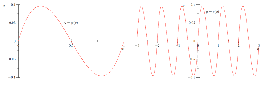
Definir\(\varphi:[0,1] \rightarrow \mathbb{R}\) por\(\varphi(x)=x(2 x-1)(x-1) .\) Definir\(\rho: \mathbb{R} \rightarrow \mathbb{R}\) por\(\rho(x)=6 x^{2}-6 x+1 .\) Entonces

\[\varphi(x)=2 x^{3}-3 x^{2}+x,\]

así que\(\varphi^{\prime}(x)=\rho(x)\) para todos\(x \in(0,1) .\) Siguiente definir\(s: \mathbb{R} \rightarrow \mathbb{R}\) por\(s(x)=\varphi(x-\lfloor x\rfloor)\). Ver Figura\(\PageIndex{1}\) para las gráficas de\(\varphi\) y\(s .\) Entonces para cualquiera\(n \in \mathbb{Z}\) y\(n<x<n+1\),

\[s^{\prime}(x)=\rho(x-n)=\rho(x-\lfloor x\rfloor).\]

Además, si\(x\) es un número entero,

\[\begin{aligned} \lim _{h \rightarrow 0^{+}} \frac{s(x+h)-s(x)}{h} &=\lim _{h \rightarrow 0^{+}} \frac{\varphi(h)}{h} \\ &=\lim _{h \rightarrow 0^{+}} \frac{h(2 h-1)(h-1)}{h} \\ &=\lim _{h \rightarrow 0^{+}}(2 h-1)(h-1) \\ &=1 \end{aligned}\]

y

\[\begin{aligned} \lim _{h \rightarrow 0^{-}} \frac{s(x+h)-s(x)}{h} &=\lim _{h \rightarrow 0^{-}} \frac{\varphi(h+1)}{h} \\ &=\lim _{h \rightarrow 0^{-}} \frac{(h+1)(2 h+1) h}{h} \\ &=\lim _{h \rightarrow 0^{-}}(h+1)(2 h+1) \\ &=1. \end{aligned}\]

Figura\(\PageIndex{1}\): Gráficas de\(y=\varphi(x)\) y\(y=s(x)\)

Así,\(s^{\prime}(x)=1=\rho(x-\lfloor x\rfloor)\) cuando\(x\) es un número entero, y así\(s^{\prime}(x)=\rho(x-\lfloor x\rfloor)\) para todos\(x \in \mathbb{R} .\)

Ahora\(\rho(x)=0\) si y solo si\(x=\frac{3-\sqrt{3}}{6}\) o\(x=\frac{3+\sqrt{3}}{6} .\) desde\(\varphi(0)=0\),\(\varphi\left(\frac{3-\sqrt{3}}{6}\right)=\frac{1}{6 \sqrt{3}}, \varphi\left(\frac{3+\sqrt{3}}{6}\right)=-\frac{1}{6 \sqrt{3}},\) y\(\varphi(1)=0,\) vemos que\(\varphi\) alcanza una

valor máximo de\(\frac{1}{6 \sqrt{3}}\) y un valor mínimo de\(-\frac{1}{6 \sqrt{3}} .\) Por lo tanto para cualquier\(n \in \mathbb{Z}\),

\[s((n, n+1))=\left[-\frac{1}{6 \sqrt{3}}, \frac{1}{6 \sqrt{3}}\right].\]

También,\(\rho^{\prime}(x)=12 x-6,\) así\(\rho^{\prime}(x)=0\) si y sólo si\(x=\frac{1}{2} .\) desde\(\rho(0)=1\),\(\rho\left(\frac{1}{2}\right)=-\frac{1}{2},\) y\(\rho(1)=1,\) vemos que\(\rho\) alcanza un valor máximo de 1 y un v,

\[s^{\prime}((n, n+1))=\left[-\frac{1}{2}, 1\right].\]

Se deduce de lo anterior, de la misma manera que el resultado en Ejemplo\(5.1 .7,\) que ni la función\(\sigma(x)=s\left(\frac{1}{x}\right)\) ni la función\(g(x)=s^{\prime}\left(\frac{1}{x}\right)\) tienen un límite como\(x\) aproximaciones\(0 .\)

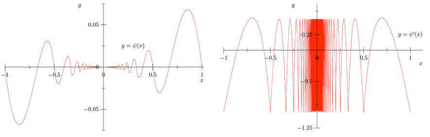
Por último, definir\(\psi: \mathbb{R} \rightarrow \mathbb{R}\) por

\[\psi(x)=\left\{\begin{array}{ll}{x^{2} s\left(\frac{1}{x}\right),} & {\text { if } x \neq 0,} \\ {0,} & {\text { if } x=0.}\end{array}\right.\]

Para\(x \neq 0,\) nosotros tenemos

\[\psi^{\prime}(x)=x^{2} s^{\prime}\left(\frac{1}{x}\right)\left(-\frac{1}{x^{2}}\right)+2 x s\left(\frac{1}{x}\right)=-s^{\prime}\left(\frac{1}{x}\right)+2 x s\left(\frac{1}{x}\right).\]

En\(0,\) tenemos

\[\begin{aligned} \psi^{\prime}(0) &=\lim _{h \rightarrow 0} \frac{\psi(0+h)-\psi(0)}{h} \\ &=\lim _{h \rightarrow 0} \frac{h^{2} s\left(\frac{1}{h}\right)}{h} \\ &=\lim _{h \rightarrow 0} h s\left(\frac{1}{h}\right) \\ &=0, \end{aligned}\]

donde el límite final se desprende del teorema squeeze y el hecho de que\(s\) está acotado. De ahí que veamos que\(\psi\) es continuo\(\mathbb{R}\) y diferenciable\(\mathbb{R},\) pero no\(\psi^{\prime}\) es continuo ya que\(\psi^{\prime}(x)\) no tiene límite como\(x\) enfoques\(0 .\) Ver Figura\(\PageIndex{1}\) para las gráficas de\(\psi\) y\(\psi^{\prime} .\)

Figura\(\PageIndex{2}\): Gráficas de\(y=\psi(x)\) y\(y=\psi^{\prime}(x)\).

Ejercicio\(\PageIndex{3}\)

\(s\)Sea como arriba y defina\(g: \mathbb{R} \rightarrow \mathbb{R}\) por

\[g(x)=\left\{\begin{array}{ll}{x^{4} s\left(\frac{1}{x}\right),} & {\text { if } x \neq 0} \\ {0,} & {\text { if } x=0.}\end{array}\right.\]

Demostrar que\(g\) es diferenciable en\(\mathbb{R}\) y que\(g^{\prime}\) es continuo en\(\mathbb{R}\).