3.6: Números catalanes

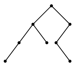
Un árbol binario enraizado es un tipo de gráfico que es particularmente interesante en algunas áreas de la informática. Un típico árbol binario enraizado se muestra en la Figura\(\PageIndex{1}\). La raíz es el vértice más alto. Los vértices por debajo de un vértice y conectados a él por un borde son los hijos del vértice. Es un árbol binario porque todos los vértices tienen 0, 1 o 2 hijos. ¿Cuántos árboles binarios enraizados diferentes hay con\(n\) vértices?

Figura\(\PageIndex{1}\): Un árbol binario enraizado.

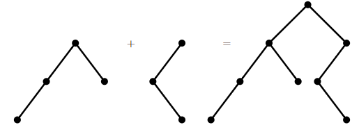
Denotemos este número por\(C_n\); estos son los números catalanes. Para mayor comodidad, permitimos que un árbol binario enraizado esté vacío, y dejar\(C_0=1\). Entonces es fácil ver eso\(C_1=1\) y\(C_2=2\), y no es difícil verlo\(C_3=5\). Observe que cualquier árbol binario enraizado en al menos un vértice puede verse como dos árboles binarios (posiblemente vacíos) unidos en un nuevo árbol introduciendo un nuevo vértice raíz y convirtiendo a los hijos de esta raíz en las dos raíces de los árboles originales; ver Figura\(\PageIndex{2}\). (Para hacer del árbol vacío un hijo del nuevo vértice, simplemente no haga nada, es decir, omita al hijo correspondiente).

Figura\(\PageIndex{2}\): Producir un nuevo árbol a partir de árboles más pequeños.

Así, para hacer todos los árboles binarios posibles con\(n\) vértices, comenzamos con un vértice raíz, y luego para sus dos hijos insertamos árboles binarios enraizados en\(k\) y\(l\) vértices, con\(k+l=n-1\), para todas las elecciones posibles de los árboles más pequeños. Ahora podemos escribir

\[ C_n=\sum_{i=0}^{n-1} C_iC_{n-i-1}. \nonumber \]

For example, since we know that \(C_0=C_1=1\) and \(C_2=2\),

\[ C_3 = C_0C_2 + C_1C_1+C_2C_0 = 1\cdot2 + 1\cdot1 + 2\cdot1 = 5, \nonumber \]

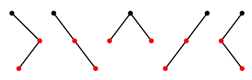
as mentioned above. Once we know the trees on 0, 1, and 2 vertices, we can combine them in all possible ways to list the trees on 3 vertices, as shown in Figure \(\PageIndex{3}\). Note that the first two trees have no left child, since the only tree on 0 vertices is empty, and likewise the last two have no right child.

Figure \(\PageIndex{3}\): The 3-vertex binary rooted trees.

Now we use a generating function to find a formula for \(C_n\). Let \(f=\sum_{i=0}^\infty C_ix^i\). Now consider \(f^2\): the coefficient of the term \(x^n\) in the expansion of \(f^2\) is \(\sum_{i=0}^{n} C_iC_{n-i}\), corresponding to all possible ways to multiply terms of \(f\) to get an \(x^n\) term: \[ C_0\cdot C_nx^n + C_1x\cdot C_{n-1}x^{n-1} + C_2x^2\cdot C_{n-2}x^{n-2} +\cdots+C_nx^n\cdot C_0. \nonumber\] Now we recognize this as precisely the sum that gives \(C_{n+1}\), so \(f^2 = \sum_{n=0}^\infty C_{n+1}x^n\). If we multiply this by \(x\) and add 1 (which is \(C_0\)) we get exactly \(f\) again, that is, \(xf^2+1=f\) or \(xf^2-f+1=0\); here 0 is the zero function, that is, \(xf^2-f+1\) is 0 for all x. Using the quadratic formula,

\[ f={1\pm\sqrt{1-4x}\over 2x}, \nonumber \]

as long as \(x\not=0\). It is not hard to see that as \(x\) approaches 0,

\[ {1+\sqrt{1-4x}\over 2x} \nonumber\]

goes to infinity while

\[ {1-\sqrt{1-4x}\over 2x}\nonumber \]

goes to 1. Since we know \(f(0)=C_0=1\), this is the \(f\) we want.

Now by Newton's Binomial Theorem, we can expand

\[ \sqrt{1-4x} = (1+(-4x))^{1/2} =\sum_{n=0}^\infty {1/2\choose n}(-4x)^n.\nonumber \]

Then

\[ {1-\sqrt{1-4x}\over 2x} = \sum_{n=1}^\infty -{1\over 2}{1/2\choose n}(-4)^nx^{n-1} = \sum_{n=0}^\infty -{1\over 2}{1/2\choose n+1}(-4)^{n+1}x^n. \nonumber \]

Expanding the binomial coefficient \(1/2\choose n+1\) and reorganizing the expression, we discover that

\[ C_n = -{1\over 2}{1/2\choose n+1}(-4)^{n+1} = {1\over n+1}{2n\choose n}.\nonumber \]

In Exercise 1.E.3.7 in Section 1.E, we saw that the number of properly matched sequences of parentheses of length \(2n\) is \({2n\choose n}-{2n\choose n+1}\), and called this \(C_n\). It is not difficult to see that

\[ {2n\choose n}-{2n\choose n+1}={1\over n+1}{2n\choose n},\nonumber \]

so the formulas are in agreement.

Temporarily let \(A_n\) be the number of properly matched sequences of parentheses of length \(2n\), so from the exercise we know \(A_n={2n\choose n}-{2n\choose n+1}\). It is possible to see directly that \(A_0=A_1=1\) and that the numbers \(A_n\) satisfy the same recurrence relation as do the \(C_n\), which implies that \(A_n=C_n\), without manipulating the generating function.

There are many counting problems whose answers turns out to be the Catalan numbers. Enumerative Combinatorics: Volume 2, by Richard Stanley, contains a large number of examples.

Contributors and Attributions

• Template:ContribGuichard