12.3: Tamaños Relativos de Conjuntos

Hemos definido un conjunto\(A\) para que sea finito cuando podamos contar sus elementos emparejándolos bijectivamente con los elementos de algún conjunto de conteo\(\mathbb{N}_{<m}\text{.}\) Y en este caso, definiendo\(\vert A \vert = m\text{,}\) estamos declarando que\(A\) tiene el mismo “tamaño” que\(\mathbb{N}_{<m}\text{.}\)

Ampliando esta idea, podemos pensar en cada bijección como usar los elementos de un conjunto para “contar” los elementos de otro.

Definición: Mismo tamaño

conjuntos\(A\) y\(B\) para los que existe una bijección\(A \to B\)

Hecho\(\PageIndex{1}\): Symmetry of size.

Si\(B\) tiene el mismo tamaño que\(A\text{,}\) entonces\(A\) tiene el mismo tamaño que\(B\text{.}\)

Comprobante.

Si\(f: A \rightarrow B\) es una biyección, entonces también lo es\(f^{-1} : B \rightarrow A\text{.}\)

Hecho\(\PageIndex{2}\): Transitivity of size.

Si\(A\) tiene el mismo tamaño que\(B\) y\(B\) tiene el mismo tamaño que\(C\text{,}\) entonces\(A\) tiene el mismo tamaño que\(C\text{.}\)

Comprobante.

Esto le queda a usted como Ejercicio 12.6.5.

Esperamos que nuestra noción general del mismo tamaño coincida con solo contar elementos de conjuntos finitos y obtener el mismo resultado.

Hecho\(\PageIndex{3}\): Finite sets with equal cardinality have the same size.

Asumir\(A\) y\(B\) son conjuntos finitos. Entonces\(\vert A \vert = \vert B \vert\) si y solo si\(A\) y\(B\) tienen el mismo tamaño.

Comprobante.

Asumir igual cardinalidad, mostrar el mismo tamaño.

Asumir\(\vert A \vert = \vert B \vert = m\text{.}\) Entonces por definición existen bijecciones\(f: \mathbb{N}_{<m} \rightarrow A\) y\(g: \mathbb{N}_{<m} \rightarrow B\text{.}\) Ahora\(g \circ f^{-1}\) es una bijección\(A \to B\text{,}\) así\(A\) y\(B\) tienen el mismo tamaño según la definición técnica.

Asumir el mismo tamaño, mostrar igual cardinalidad.

Asumir\(A\) y\(B\) tener el mismo tamaño. Entonces por definición existe una bijección\(f: A \rightarrow B\text{.}\) Ahora, también hemos asumido que\(A\) es finito, entonces existe una bijección\(g: \mathbb{N}_{<m} \rightarrow A\text{,}\) donde\(m = \vert A \vert\text{.}\) Entonces\(f \circ g: \mathbb{N}_{<m} \rightarrow B\) es una bijección que demuestra\(\vert B \vert = m\) también.

Advertencia

Tu intuición puede fallarte al considerar “tamaños” de conjuntos infinitos. En particular, es posible tener\(\vert A \vert = \vert B \vert = \infty\text{,}\) dónde\(A\) y\(B\) no tener el mismo tamaño.

 

Ejemplo\(\PageIndex{1}\): Sets of integers and natural numbers have the same size.

A pesar de\(\mathbb{Z}\) que\(\mathbb{N} \subsetneqq \mathbb{Z}\text{,}\)\(\mathbb{N}\) y tienen el mismo tamaño! A continuación se define una biyección\(f: \mathbb{N} \rightarrow \mathbb{Z}\text{.}\)

\(n\)	\(0\)	\(1\)	\(2\)	\(3\)	\(4\)	\(\cdots\)
\(f(n)\)	\(0\)	\(-1\)	\(1\)	\(-2\)	\(2\)	\(\cdots\)

Esta biyección se puede expresar por la fórmula

\ begin {equation*} f (n) =\ begin {cases}\ dfrac {m} {2}, & m\ text {par},\\ -\ dfrac {m+1} {2}, & m\ text {impar}. \ end {cases}\ end {ecuación*}

Ejemplo\(\PageIndex{2}\): Sets of real numbers and natural numbers do not have the same size.

En el Capítulo 13, vamos a ver que a pesar de que\(\vert \mathbb{N} \vert = \vert \mathbb{R} \vert = \infty\text{,}\) los conjuntos\(\mathbb{N}\) y\(\mathbb{R}\) no tienen el mismo tamaño!

Ejemplo\(\PageIndex{3}\): Intervals of real numbers of different lengths have the same size.

Recordemos del cálculo de primer año que para\(a,b \in \mathbb{R}\) con\(a \lt b\text{,}\) definimos el intervalo abierto de\(a\)\(b\) a ser el conjunto de todos los números reales estrictamente entre\(a\) y\(b\text{:}\)

\ begin {ecuación*} (a, b) =\ {x\ in\ mathbb {R}\ vert a\ lt x\ lt b\}\ texto {.} \ end {ecuación*}

Figura\(\PageIndex{1}\): Intervalo en la recta numérica real.

Resulta que, aunque puedan tener diferentes longitudes, ¡el intervalo\((a,b)\) y el intervalo unitario\((0,1)\) tienen el mismo tamaño! (Es decir, de alguna manera contienen el mismo “número” de números.)

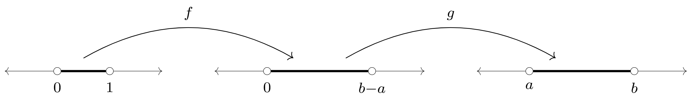
Construir una biyección\((0,1)\to(a,b)\) en dos pasos.

1. El mapa
   \ begin {alinear*} f\ colon (0,1) &\ to (0, b-a),\\ x &\ mapsto (b-a) x,\ end {align*}
   es una biyección. (¡Cheque!)
2. El mapa
   \ begin {alinear*} g\ colon (0, b-a) &\ to (a, b),\\ x &\ mapsto x+a,\ end {align*}
   es una biyección. (¡Cheque!)

Entonces\(g\circ f: (0,1) \rightarrow (a,b)\) es una biyección.

Figura\(\PageIndex{2}\): Escalar y traducir el intervalo unitario a otro intervalo.

Ejemplo\(\PageIndex{4}\): A punctured circle has the same size as \(\mathbb{R}\).

Definir

\ begin {alinear*} S & =\ {(x, y)\ in\ mathbb {R} ^2\ vert x^2 + (y-\ dfrac {1} {2}) ^2 =\ dfrac {1} {4}\}\ texto {,} &\ hat {S} & = S\ setmenos\ {(0,1)\}\ texto {.} \ end {align*}
Aquí,\(S\) hay un círculo en el plano con radio\(\dfrac{1}{2}\) y centro\((0,\dfrac{1}{2})\text{,}\) y\(\hat{S}\) es el círculo\(S\) “perforado” en el “polo norte”.

Afirmamos que\(\hat{S}\) tiene el mismo tamaño que\(\mathbb{R}\text{.}\) Construir una bijección\(\hat{S}\to\mathbb{R}\) en dos pasos.

1. Dejar\(X\) representar el\(x\) eje -en el plano, i.e.

\ begin {ecuación*} X =\ {(x,0)\ vert x\ in\ mathbb {R}\}\ subseteq\ mathbb {R} ^2\ text {.} \ end {equation*}
Dejar\(f: \hat{S} \rightarrow X\) definirse de la siguiente manera: para\((x,y)\in \hat{S}\text{,}\) let\(f(x,y)\) ser la\(x\) -intercepción de la línea a través de puntos\((0,1),(x,y)\text{.}\)

Figura\(\PageIndex{3}\): Proyectar el círculo perforado sobre la línea numérica real.

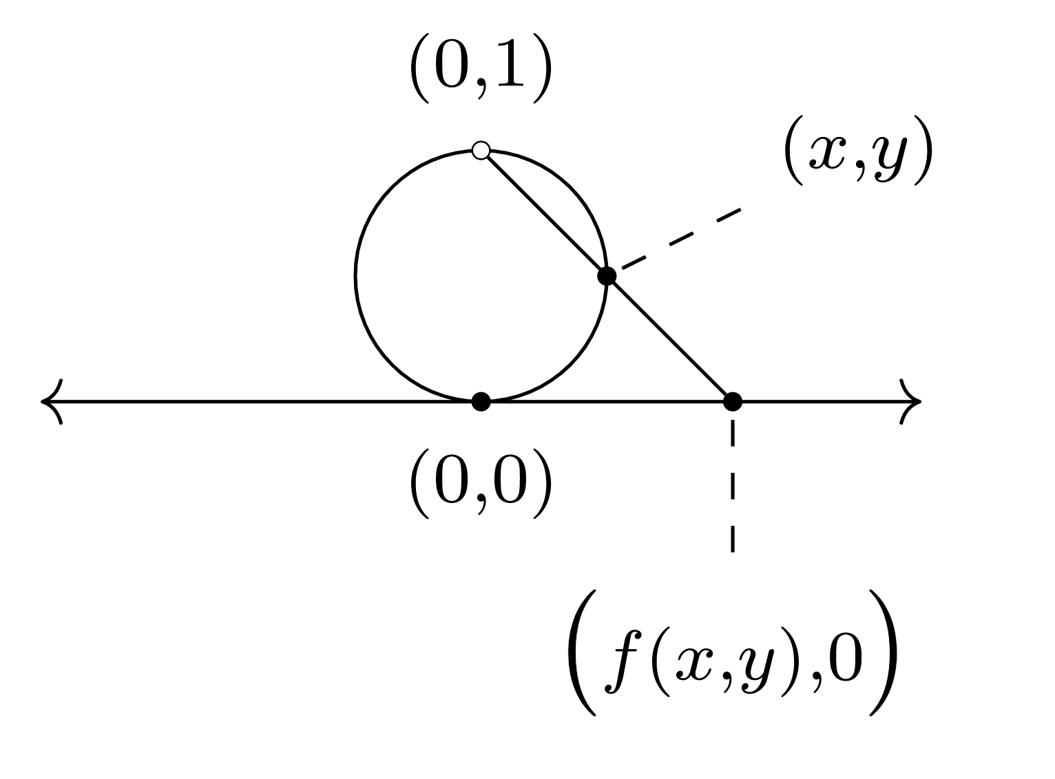
Entonces\(f\) es una biyección. (¡Cheque!)

2. También tenemos una bijección\(g: X \rightarrow \mathbb{R}\) por\(g(x,0) = x\text{.}\)

Por lo tanto, la composición\(g\circ f : \hat{S} \rightarrow \mathbb{R}\) es una biyección.

Ejemplo\(\PageIndex{5}\): Every interval of real numbers has the same size as the entire set of real numbers.

Ejemplo\(\PageIndex{3}\) y Ejemplo se\(\PageIndex{4}\) pueden combinar para demostrar que cada intervalo\((a,b)\) de longitud finita de números reales tiene el mismo tamaño que el conjunto completo\(\mathbb{R}\) de números reales. Ver Ejercicio 12.6.6.