3.1: El Algoritmo Euclidiana

Última actualización
Guardar como PDF

Page ID: 111475

$ \newcommand{\vecs}[1]{\overset { \scriptstyle \rightharpoonup} {\mathbf{#1}} } $ $ \newcommand{\vecd}[1]{\overset{-\!-\!\rightharpoonup}{\vphantom{a}\smash {#1}}} $$\newcommand{\id}{\mathrm{id}}$ $ \newcommand{\Span}{\mathrm{span}}$ $ \newcommand{\kernel}{\mathrm{null}\,}$ $ \newcommand{\range}{\mathrm{range}\,}$ $ \newcommand{\RealPart}{\mathrm{Re}}$ $ \newcommand{\ImaginaryPart}{\mathrm{Im}}$ $ \newcommand{\Argument}{\mathrm{Arg}}$ $ \newcommand{\norm}[1]{\| #1 \|}$ $ \newcommand{\inner}[2]{\langle #1, #2 \rangle}$ $ \newcommand{\Span}{\mathrm{span}}$ $\newcommand{\id}{\mathrm{id}}$ $ \newcommand{\Span}{\mathrm{span}}$ $ \newcommand{\kernel}{\mathrm{null}\,}$ $ \newcommand{\range}{\mathrm{range}\,}$ $ \newcommand{\RealPart}{\mathrm{Re}}$ $ \newcommand{\ImaginaryPart}{\mathrm{Im}}$ $ \newcommand{\Argument}{\mathrm{Arg}}$ $ \newcommand{\norm}[1]{\| #1 \|}$ $ \newcommand{\inner}[2]{\langle #1, #2 \rangle}$ $ \newcommand{\Span}{\mathrm{span}}$$\newcommand{\AA}{\unicode[.8,0]{x212B}}$

Lema 3.1

En el algoritmo de división de Definition2.4, tenemos$\gcd(r_{1},r_{2}) = \gcd(r_{2}, r_{3})$.

Prueba: Por un lado, tenemos$r_{1} = r_{2}q_{2}+r_{3}$, y así cualquier divisor común de$r_{2}$ y también$r_{3}$ debe ser un divisor de$r_{1}$ (y de$r_{2}$). Viceversa$r_{1}-r_{2}q_{2} = r_{3}$, ya que, tenemos ese cualquier divisor común de$r_{1}$ y también$r_{2}$ debe ser un divisor de$r_{3}$ (y de$r_{2}$).

Así, al calcular$r_{3}$, el residuo de$r_{1}$ módulo$r_{2}$, hemos simplificado el cómputo de$\gcd (r_{1}, r_{2})$. Esto se debe a que$r_{3}$ es estrictamente menor (en valor absoluto) que ambos$r_{1}$ y$r_{2}$. A su vez, el cálculo de$\gcd (r_{2}, r_{3})$ puede simplificarse de manera similar, y así se puede repetir el proceso. Dado que la$r_{i}$ forma una secuencia decreciente monótona en$\mathbb{N}$, este proceso debe terminar cuando$r_{n}+1 = 0$ después de un número finito de pasos. Entonces tenemos$gcd(r_{1},r_{2}) = gcd(r_{n},0) = r_{n}$.

Corolario 3.2

Dado$r_{1} > r_{2} > 0$, aplicar el algoritmo de división hasta$r_{n} > r_{n+1} = 0$. Entonces$\gcd (r_{1}, r_{2}) = \gcd(r_{n}, 0) = r_{n}$. Como$r_{i}$ es decreciente, el algoritmo siempre termina.

Definición 3.3

La aplicación repetida del algoritmo de división para calcular$\gcd(r_{1}, r_{2})$ se denomina algoritmo euclidiano.

Ahora damos un marco para reducir el desorden de estos cálculos repetidos. Supongamos que queremos calcular$\gcd(188, 158)$. Hacemos los siguientes cálculos:

\[188 = 158·1+30 \nonumber\]

\[158 = 30·5+8 \nonumber\]

\[30 = 8·3+6 \nonumber\]

\[8 = 6·1+2 \nonumber\]

\[6 = 2·3+0 \nonumber\]

Eso lo vemos$\gcd(188,158) = 2$. Los números que multiplican el$r_{i}$ son los cocientes del algoritmo de división (ver la prueba de Lemma 2.3). Si los llamamos$q_{i-1}$, el cómputo se ve de la siguiente manera:

\[\begin{array} {c} {r_{1} = r_{2} q_{2}+r_{3}}\\ {r_{2} = r_{3} q_{3}+r_{4}}\\ {\vdots}\\ {r_{n-3} = r_{n-2} q_{n-2}+r_{n-3}}\\ {r_{n-2} = r_{n-1} q_{n-1}+r_{n-2}}\\ {r_{n-1} = r_{n} q_{n}+0} \end{array}\]

donde usamos la convención que$r_{n+1} = 0$ mientras$r_{n} \ne 0$. Observe que con esa convención, (3.1) consiste en$n-1$ pasos. Una forma mucho más concisa (en parte basada en una sugerencia de Katahdin [16]) para renderizar este cálculo es la siguiente.

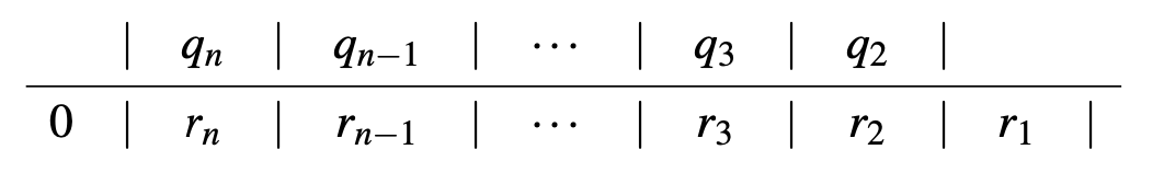
$Screen Shot 2021-04-21 at 3.48.54 PM.png$

Así, cada paso$r_{i+1} |r_{i}|$ es similar a la división larga habitual, salvo que su cociente$q_{i+1}$ se coloca arriba$r_{i+1}$ (y no arriba$r_{i}$), mientras que su resto$r_{i+2}$ se coloca todo el camino a la izquierda de$r_{i+1}$. El ejemplo que elaboramos antes de ahora parece:

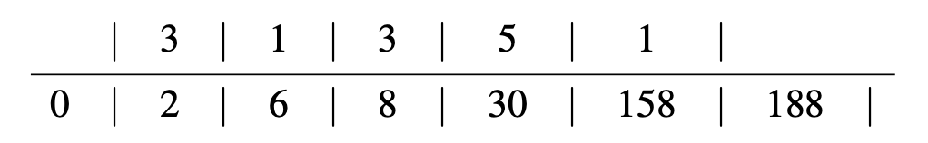
$Screen Shot 2021-04-21 en 3.50.42 PM.png$

Hay una hermosa visualización de este proceso esbozado en el ejercicio 3.4.