3.10:3. 10- Solución del problema de los mínimos cuadrados
- Page ID
- 119044

\( \newcommand{\vecs}[1]{\overset { \scriptstyle \rightharpoonup} {\mathbf{#1}} } \)
\( \newcommand{\vecd}[1]{\overset{-\!-\!\rightharpoonup}{\vphantom{a}\smash {#1}}} \)
\( \newcommand{\id}{\mathrm{id}}\) \( \newcommand{\Span}{\mathrm{span}}\)
( \newcommand{\kernel}{\mathrm{null}\,}\) \( \newcommand{\range}{\mathrm{range}\,}\)
\( \newcommand{\RealPart}{\mathrm{Re}}\) \( \newcommand{\ImaginaryPart}{\mathrm{Im}}\)
\( \newcommand{\Argument}{\mathrm{Arg}}\) \( \newcommand{\norm}[1]{\| #1 \|}\)
\( \newcommand{\inner}[2]{\langle #1, #2 \rangle}\)
\( \newcommand{\Span}{\mathrm{span}}\)
\( \newcommand{\id}{\mathrm{id}}\)
\( \newcommand{\Span}{\mathrm{span}}\)
\( \newcommand{\kernel}{\mathrm{null}\,}\)
\( \newcommand{\range}{\mathrm{range}\,}\)
\( \newcommand{\RealPart}{\mathrm{Re}}\)
\( \newcommand{\ImaginaryPart}{\mathrm{Im}}\)
\( \newcommand{\Argument}{\mathrm{Arg}}\)
\( \newcommand{\norm}[1]{\| #1 \|}\)
\( \newcommand{\inner}[2]{\langle #1, #2 \rangle}\)
\( \newcommand{\Span}{\mathrm{span}}\) \( \newcommand{\AA}{\unicode[.8,0]{x212B}}\)
\( \newcommand{\vectorA}[1]{\vec{#1}} % arrow\)
\( \newcommand{\vectorAt}[1]{\vec{\text{#1}}} % arrow\)
\( \newcommand{\vectorB}[1]{\overset { \scriptstyle \rightharpoonup} {\mathbf{#1}} } \)
\( \newcommand{\vectorC}[1]{\textbf{#1}} \)
\( \newcommand{\vectorD}[1]{\overrightarrow{#1}} \)
\( \newcommand{\vectorDt}[1]{\overrightarrow{\text{#1}}} \)
\( \newcommand{\vectE}[1]{\overset{-\!-\!\rightharpoonup}{\vphantom{a}\smash{\mathbf {#1}}}} \)
\( \newcommand{\vecs}[1]{\overset { \scriptstyle \rightharpoonup} {\mathbf{#1}} } \)
\( \newcommand{\vecd}[1]{\overset{-\!-\!\rightharpoonup}{\vphantom{a}\smash {#1}}} \)
View Solución del problema de mínimos cuadrados por las ecuaciones normales en YouTube
El problema de los mínimos cuadrados se puede lanzar como el problema de resolver una ecuación matricial sobredeterminada\(\text{Ax} = \text{b}\) cuando no\(\text{b}\) está en el espacio de columna de\(\text{A}\). Al reemplazar\(\text{b}\) por su proyección ortogonal sobre el espacio de columna de\(\text{A}\), la solución minimiza la norma\(||\text{Ax} − \text{b}||\).
Ahora\(\text{b} = \text{b}_{\text{proj}_{\text{Col(A)}}} + (\text{b} − \text{b}_{\text{proj}_{\text{Col(A)}}})\), ¿dónde\(\text{b}_{\text{proj}_{\text{Col(A)}}}\) está la proyección de\(\text{b}\) sobre el espacio de columna de\(\text{A}\). Dado que\((\text{b} − \text{b}_{\text{proj}_{\text{Col(A)}}})\) es ortogonal al espacio de columna de\(\text{A}\), está en el espacio nulado de\(\text{A}^{\text{T}}\). Por lo tanto\(\text{A}^{\text{T}}(\text{b} − \text{b}_{\text{proj}_{\text{Col(A)}}} ) = 0\),, y paga\(\text{A}^{\text{T}}\) multiplicar\(\text{Ax} = \text{b}\) por obtener
\[\text{A}^{\text{T}}\text{Ax}=\text{A}^{\text{T}}\text{b}.\nonumber \]
Estas ecuaciones, llamadas ecuaciones normales para\(\text{Ax} = \text{b}\), determinan la solución de mínimos cuadrados para\(\text{x}\), que se puede encontrar por eliminación gaussiana. Cuando\(\text{A}\) es una\(n\) matriz\(m\) -by-, entonces\(\text{A}^{\text{T}}\text{A}\) es una\(n\) matriz\(n\) -by-, y se puede mostrar que\(\text{A}^{\text{T}}\text{A}\) es invertible cuando las columnas de\(\text{A}\) son linealmente independientes. Cuando este es el caso, se pueden reescribir las ecuaciones normales multiplicando ambos lados por\(\text{A}(\text{A}^{\text{T}}\text{A})^{−1}\) para obtener
\[\text{Ax}=\text{A}(\text{A}^{\text{T}}\text{A})^{-1}\text{A}^{\text{T}}\text{b},\nonumber \]
donde la matriz
\[\text{P}=\text{A}(\text{A}^{\text{T}}\text{A})^{-1}\text{A}^{\text{T}}\nonumber \]
proyecta un vector en el espacio de columna de\(\text{A}\). Es fácil probarlo\(\text{P}^2 = \text{P}\), lo que establece que dos proyecciones son iguales a una. Tenemos
\[\begin{aligned}\text{P}^2&=(\text{A}(\text{A}^{\text{T}}\text{A})^{-1}\text{A}^{\text{T}})(\text{A}(\text{A}^{\text{T}}\text{A})^{-1}\text{A}^{\text{T}}) \\ &=\text{A}\left[(\text{A}^{\text{T}}\text{A})^{-1}(\text{A}^{\text{T}}\text{A})\right](\text{A}^{\text{T}}\text{A})^{-1}\text{A}^{\text{T}} \\ &=\text{A}(\text{A}^{\text{T}}\text{A})^{-1}\text{A}^{\text{T}}=P.\end{aligned} \nonumber \]
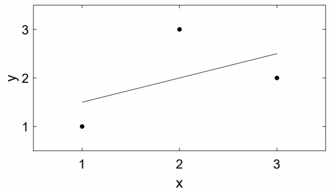
Como ejemplo, considere el problema de los mínimos cuadrados del juguete de ajustar una línea a través de los tres puntos de datos\((1, 1),\: (2, 3)\) y\((3, 2)\). Con la línea dada por\(y = \beta_0 + \beta_1x\), el sistema sobredeterminado de ecuaciones viene dado por
\[\left(\begin{array}{cc}1&1\\1&2\\1&3\end{array}\right)\left(\begin{array}{c}\beta_0\\ \beta_1\end{array}\right)=\left(\begin{array}{c}1\\3\\2\end{array}\right).\nonumber \]
La solución de mínimos cuadrados se determina resolviendo
\[\left(\begin{array}{ccc}1&1&1\\1&2&3\end{array}\right)\left(\begin{array}{cc}1&1\\1&2\\1&3\end{array}\right)\left(\begin{array}{c}\beta_0\\ \beta_1\end{array}\right)=\left(\begin{array}{ccc}1&1&1\\1&2&3\end{array}\right)\left(\begin{array}{c}1\\3\\2\end{array}\right),\nonumber \]
o
\[\left(\begin{array}{cc}3&6\\6&14\end{array}\right)\left(\begin{array}{c}\beta_0 \\ \beta_1\end{array}\right)=\left(\begin{array}{c}6\\13\end{array}\right).\nonumber \]
Podemos resolver ya sea invirtiendo directamente la matriz de dos por dos o usando la eliminación gaussiana. Invirtiendo la matriz de dos por dos, tenemos
\[\left(\begin{array}{c}\beta_0 \\ \beta_1\end{array}\right)=\frac{1}{6}\left(\begin{array}{rr}14&-6 \\ -6&3\end{array}\right)\left(\begin{array}{c}6\\13\end{array}\right)=\left(\begin{array}{c}1\\1/2\end{array}\right),\nonumber \]
de manera que la línea de mínimos cuadrados viene dada por
\[y=1+\frac{1}{2}x.\nonumber \]
A continuación se muestra la gráfica de los datos y la línea.