10.1: Distintos valores propios reales

Ilustramos el método de solución con el ejemplo.

Ejemplo: Encuentra la solución general de\(\dot{x}_{1}=x_{1}+x_{2}, \dot{x}_{2}=4 x_{1}+x_{2}\).

Ver tutorial en YouTube

La ecuación a resolver puede ser reescrita en forma de matriz como

\[\frac{d}{d t}\left(\begin{array}{l} x_{1} \\ x_{2} \end{array}\right)=\left(\begin{array}{ll} 1 & 1 \\ 4 & 1 \end{array}\right)\left(\begin{array}{l} x_{1} \\ x_{2} \end{array}\right) \nonumber \]

o en mano corta como Ecuación\ ref {10.2}.

Tomamos como nuestro ansatz\(x(t)=v e^{\lambda t}\), donde\(v\) y\(\lambda\) somos independientes de\(t\). Tras la sustitución en la Ecuación\ ref {10.2}, obtenemos

\[\lambda \mathrm{v} e^{\lambda t}=\mathrm{Av}^{\lambda t} \nonumber \]

y al cancelar lo exponencial, obtenemos el problema del valor propio

\[\mathrm{Av}=\lambda \mathrm{v} . \nonumber \]

Encontrando la ecuación característica usando la ecuación\ ref {5.4}, tenemos

\[\begin{aligned} 0 &=\operatorname{det}(\mathrm{A}-\lambda \mathrm{I}) \\ &=\lambda^{2}-2 \lambda-3 \\ &=(\lambda-3)(\lambda+1) \end{aligned} \nonumber \]

Por lo tanto, los dos valores propios son\(\lambda_{1}=3\) y\(\lambda_{2}=-1\).

Para determinar los vectores propios correspondientes, sustituimos los autovalores sucesivamente en

\[(\mathrm{A}-\lambda \mathrm{I}) \mathrm{v}=0 . \nonumber \]

Escribiremos los vectores propios correspondientes\(v_{1}\) y\(v_{2}\) usando la notación matricial

\[\left(\begin{array}{ll} \mathrm{v}_{1} & \mathrm{v}_{2} \end{array}\right)=\left(\begin{array}{ll} v_{11} & v_{12} \\ v_{21} & v_{22} \end{array}\right), \nonumber \]

donde los componentes de\(v_{1}\) y\(v_{2}\) se escriben con subíndices correspondientes a la primera y segunda columnas de una matriz de 2 por 2.

Para\(\lambda_{1}=3\), y autovector desconocido\(v_{1}\), tenemos de Ecuación\ ref {10.5}

\[\begin{gathered} -2 v_{11}+v_{21}=0 \\ 4 v_{11}-2 v_{21}=0 \end{gathered} \nonumber \]

Claramente, la segunda ecuación es solo la primera ecuación multiplicada por\(-2\), por lo que sólo una ecuación es linealmente independiente. Esto siempre será cierto, así que para el caso 2 -por-2 solo necesitamos considerar la primera fila de la matriz. Por lo tanto, el primer vector propio satisface\(v_{21}=2 v_{11}\). Recordemos que un vector propio solo es único hasta la multiplicación por una constante: por lo tanto, podemos tomarlo\(v_{11}=1\) por conveniencia.

Para\(\lambda_{2}=-1\), y eigenvector\(v_{2}=\left(v_{12}, v_{22}\right)^{T}\), tenemos de Ecuación\ ref {10.5}

\[2 v_{12}+v_{22}=0, \nonumber \]

para que\(v_{22}=-2 v_{12}\). Aquí, tomamos\(v_{12}=1\).

Por lo tanto, nuestros valores propios y vectores propios están dados por

\[\lambda_{1}=3, \mathrm{v}_{1}=\left(\begin{array}{l} 1 \\ 2 \end{array}\right) ; \quad \lambda_{2}=-1, \mathrm{v}_{2}=\left(\begin{array}{r} 1 \\ -2 \end{array}\right) \text {. } \nonumber \]

Usando el principio de superposición, la solución general a la oda es, por lo tanto,

\[X(t)=c_{1} v_{1} e^{\lambda_{1} t}+c_{2} v_{2} e^{\lambda_{2} t} \nonumber \]

o escribir explícitamente los componentes,

\[\begin{aligned} &x_{1}(t)=c_{1} e^{3 t}+c_{2} e^{-t} \\ &x_{2}(t)=2 c_{1} e^{3 t}-2 c_{2} e^{-t} \end{aligned} \nonumber \]

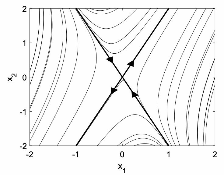
Podemos obtener una nueva perspectiva sobre la solución dibujando un retrato de fase, mostrado en la Fig. 10.1, con "\(\mathrm{x}\)-axis”\(x_{1}\) y "\(\mathrm{y}\)-axis”\(x_{2}\). Cada curva corresponde a una condición inicial diferente, y representa la trayectoria de una partícula con la velocidad dada por la ecuación diferencial. Las líneas oscuras representan trayectorias a lo largo de la dirección de los vectores propios. Si\(c_{2}=0\), el movimiento es a lo largo del vector propio\(v_{1}\) con\(x_{2}=2 x_{1}\) y el movimiento con el tiempo creciente está lejos del origen (flechas señalando) desde el valor propio\(\lambda_{1}=3>0\). Si\(c_{1}=0\), el movimiento es a lo largo del vector propio\(\mathrm{v}_{2}\) con\(x_{2}=-2 x_{1}\) y el movimiento es hacia el origen (flechas apuntando hacia adentro) desde el valor propio\(\lambda_{2}=-1<0\). Cuando los valores propios son reales y de signos opuestos, el origen se denomina punto de sillín. Casi todas las trayectorias (con la excepción de aquellas con condiciones iniciales exactamente satisfactorias\(x_{2}(0)=-2 x_{1}(0)\)) eventualmente se alejan del origen a medida que\(t\) aumenta. Cuando los valores propios son reales y del mismo signo, el origen se llama nodo. Un nodo puede ser estable (valores propios negativos) o inestable (valores propios positivos).

Figura 10.1: Retrato de fase por ejemplo con dos valores propios reales de signo opuesto.