
5.1: Las funciones trigonométricas
- Page ID
- 114541

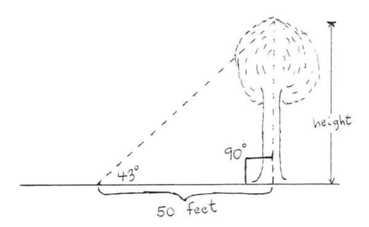
La trigonometría (de las palabras griegas que significan triángulo-medida) es la rama de las matemáticas que se ocupa de computar lados desconocidos y ángulos de triángulos. Por ejemplo, en Figura\(\PageIndex{1}\), podríamos querer medir la altura del árbol sin realmente tener que trepar al árbol. Los métodos de trigonometría nos permitirán hacerlo.
En este libro consideraremos solo la trigonometría del triángulo rectángulo. En cursos más avanzados, la trigonometría se ocupa también de otro tipo de triángulos. Aquí, sin embargo, las siguientes definiciones se aplican únicamente a los triángulos rectos.
En triángulo rectángulo\(ABC\) de la Figura\(\PageIndex{2}\),\(AC\) se llama la pierna adyacente a\(\angle A\). “Adyacente” significa “al lado”. \(BC\)se llama la pierna opuesta\(\angle A\). “Opuesto” aquí significa “más alejado de”.
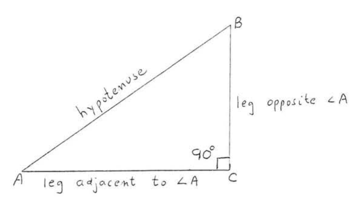
Definimos el seno, el coseno y la tangente de un ángulo agudo\(A\) en un triángulo rectángulo de la siguiente manera:
\(\begin{array} {lcl} {\text{sine } A = \dfrac{\text{leg opposite } \angle A}{\text{hypotenuse}}} & \ \ \ & {(\sin A = \dfrac{\text{opp}}{\text{hyp}})} \\ {\text{cosine } A = \dfrac{\text{leg adjacent to } \angle A}{\text{hypotenuse}}} & \ \ \ & {(\cos A = \dfrac{\text{adj}}{\text{hyp}})} \\ {\text{tangent } A = \dfrac{\text{leg opposite } \angle A}{\text{leg adjacent to } \angle A}} & \ \ \ & {(\tan A = \dfrac{\text{opp}}{\text{adj}})} \end{array}\)
El seno, el coseno y la tangente se denominan funciones trigonométricas.
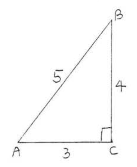
Encuentra el seno, coseno y tangente de\(\angle A\):
Solución
pierna adyacente a\(\angle A = 3\).
pierna opuesta\(\angle A = 4\).
hipotenusa = 5.
\(\sin A = \dfrac{\text{opp}}{\text{hyp}} = \dfrac{4}{5}\). \(\cos A = \dfrac{\text{adj}}{\text{hyp}} = \dfrac{3}{5}\). \(\tan A = \dfrac{\text{opp}}{\text{adj}} = \dfrac{4}{3}\).
Respuesta:\(\sin A = \dfrac{4}{5}\),\(\cos A = \dfrac{3}{5}\),\(\tan A = \dfrac{4}{3}\).
Encuentra el seno, coseno y tangente de\(\angle B\):
Solución
pierna adyacente a\(\angle B = 4\).
pierna opuesta\(\angle B = 3\).
hipotenusa = 5.
\(\sin B = \dfrac{\text{opp}}{\text{hyp}} = \dfrac{3}{5}\). \(\cos B = \dfrac{\text{adj}}{\text{hyp}} = \dfrac{4}{5}\). \(\tan B = \dfrac{\text{opp}}{\text{adj}} = \dfrac{3}{4}\).
Respuesta:\(\sin B = \dfrac{3}{5}\),\(\cos B = \dfrac{4}{5}\),\(\tan B = \dfrac{3}{4}\).
Se deben memorizar las definiciones de seno, coseno y tangente. Puede ser útil recordar el mnemotécnico “SOHCAHTOA:”

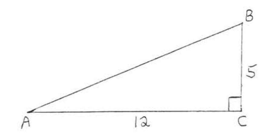
Buscar\(\sin A\),\(\cos A\), y\(\tan A\):
Solución
Para encontrar la hipotenusa, utilizamos el Teorema de Pitágoras:
\(\begin{array} {rcl} {\text{leg}^2 + \text{leg}^2} & = & {\text{hyp}^2} \\ {5^2 + 12^2} & = & {\text{hyp}^2} \\ {25 + 144} & = & {\text{hyp}^2} \\ {169} & = & {\text{hyp}^2} \\ {13} & = & {\text{hyp}} \end{array}\)
\(\sin A = \dfrac{\text{opp}}{\text{hyp}} = \dfrac{5}{13}\). \(\cos A = \dfrac{\text{adj}}{\text{hyp}} = \dfrac{12}{13}\). \(\tan A = \dfrac{\text{opp}}{\text{adj}} = \dfrac{5}{12}\).
Respuesta:\(\sin A = \dfrac{5}{13}\),\(\cos A = \dfrac{12}{13}\),\(\tan A = \dfrac{5}{12}\).
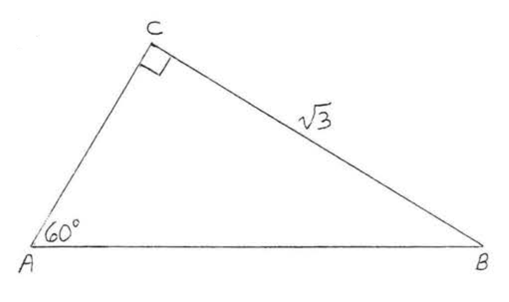
Buscar\(\sin A\),\(\cos A\), y\(\tan A\):
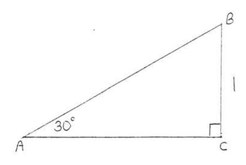
Solución
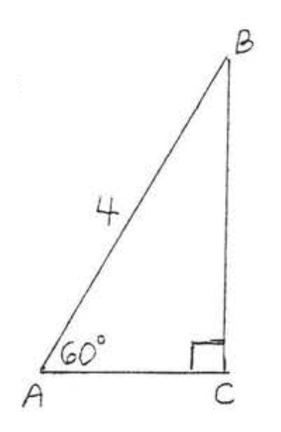
\(\triangle ABC\)es un\(30^{\circ}-60^{\circ}-90^{\circ}\) triángulo así por el Teorema 4.5.1, Sección 4.5,\(AB = \text{hyp} = 2s = 2(1) = 2\) y\(AC = L = s\sqrt{3} = (1) \sqrt{3} = \sqrt{3}\).
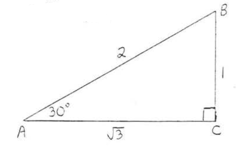
\(\sin A = \dfrac{\text{opp}}{\text{hyp}} = \dfrac{1}{2}\),\(\cos A = \dfrac{\text{adj}}{\text{hyp}} = \dfrac{\sqrt{3}}{2}\),
\(\tan A = \dfrac{\text{opp}}{\text{adj}} = \dfrac{1}{\sqrt{3}} = \dfrac{1}{\sqrt{3}} \dfrac{\sqrt{3}}{\sqrt{3}} = \dfrac{\sqrt{3}}{3}\).
Respuesta:\(\sin A = \dfrac{1}{2}\),\(\cos A = \dfrac{\sqrt{3}}{2}\),\(\tan A = \dfrac{\sqrt{3}}{3}\).
Buscar\(\sin D, \cos D\), y\(\tan D\):
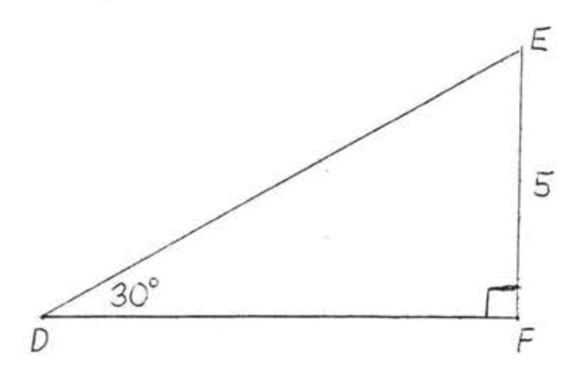
Solución
Nuevamente usando el Teorema 4.5.1, Sección 4.5,\(DE = \text{hyp} = 2s = 2(5) = 10\) y\(DF = L = s\sqrt{3} = 5\sqrt{3}\).
\(\sin D = \dfrac{\text{opp}}{\text{hyp}} = \dfrac{5}{10} = \dfrac{1}{2}\),\(\cos D = \dfrac{\text{adj}}{\text{hyp}} = \dfrac{5\sqrt{3}}{10} = \dfrac{\sqrt{3}}{2}\),\(\tan D = \dfrac{\text{opp}}{\text{adj}} = \dfrac{5}{5\sqrt{3}} = \dfrac{1}{\sqrt{3}} = \dfrac{\sqrt{3}}{3}\).
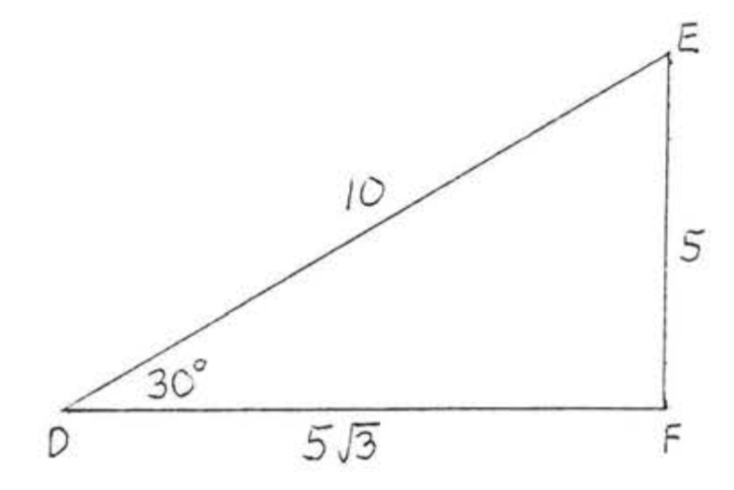
Respuesta:\(\sin D = \dfrac{1}{2}\),\(\cos D = \dfrac{\sqrt{3}}{2}\),\(\tan D = \dfrac{\sqrt{3}}{3}\).
Observe que las respuestas de Ejemplo\(\PageIndex{4}\) a Ejemplo\(\PageIndex{5}\) fueron las mismas. Esto es porque\(\angle A = \angle D = 30^{\circ}\). Los valores de las funciones trigonométricas para todos los\(30^{\circ}\) ángulos serán los mismos, La razón es que todos los triángulos rectos con un\(30^{\circ}\) ángulo son similares. Por lo tanto, sus lados son proporcionales y las relaciones trigonométricas son iguales. Lo que se sostiene para\(30^{\circ}\) los ángulos también se mantiene para otros ángulos agudos. Esto lo exponemos en el siguiente teorema:
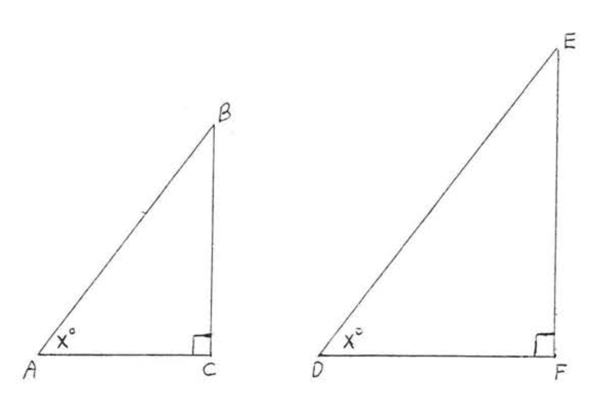
Los valores de las funciones trigonométricas para ángulos iguales son los mismos.
En la Figura\(\PageIndex{3}\), si\(\angle A = \angle D = x^{\circ}\) entonces\(\sin A = \sin D\),\(\cos A = \cos D\), y\(\tan A = \tan D\).
- Prueba
-
\(\angle A = \angle D = x^{\circ}\)y\(\angle C = \angle F = 90^{\circ}\) así\(\triangle ABC \cong \triangle DEF\) por\(AA = AA\). Por lo tanto,
\(\dfrac{BC}{EF} = \dfrac{AB}{DE}\)y\(\dfrac{AC}{DF} = \dfrac{AB}{DE}\) y\(\dfrac{BC}{EF} = \dfrac{AC}{DF}\).
Por Teorema 4.1.2, Sección 4.1, podemos intercambiar las medias de cada proporción:
\(\dfrac{BC}{AB} = \dfrac{EF}{DE}\)y\(\dfrac{AC}{AB} = \dfrac{DF}{DE}\) y\(\dfrac{BC}{AC} = \dfrac{EF}{DF}\).
Estas proporciones solo indican que
\(\sin A = \sin D\), y\(\cos A = \cos D\), y\(\tan A = \tan D\).
El teorema nos\(\PageIndex{1}\) dice que las funciones trigonométricas no dependen del triángulo particular elegido, sólo del número de grados en el ángulo. Si queremos encontrar los valores trigonométricos de un ángulo, podemos elegir cualquier triángulo rectángulo que contenga el ángulo que sea conveniente de usar.
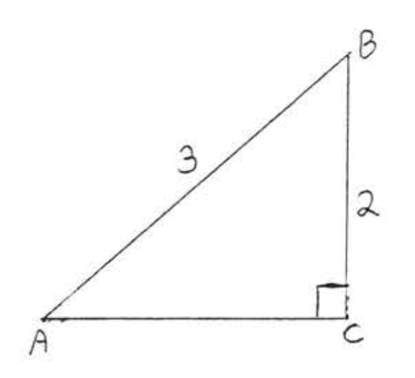
Si\(\sin A = \dfrac{12}{13}\) encuentra\(\cos A\) y\(\tan A\).
Solución
Si\(\sin A = \dfrac{\text{opp}}{\text{hyp}} = \dfrac{12}{13}\) entonces hay un triángulo rectángulo\(ABC\) que contiene\(\angle A\) con la pierna opuesta\(\angle = 12\) e hipotenusa = 13 (ver Figura\(\PageIndex{4}\)).
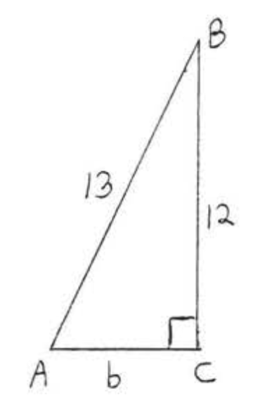
Dejar\(b =\) la pierna adyacente a\(\angle A\).
\(\begin{array} {rcl} {\text{leg}^2 + \text{leg}^2} & = & {\text{hyp}^2} \\ {b^2 + 12^2} & = & {13^2} \\ {b^2 + 144} & = & {169} \\ {-144} & \ & {-144} \\ {b^2} & = & {25} \\ {b} & = & {5} \end{array}\)
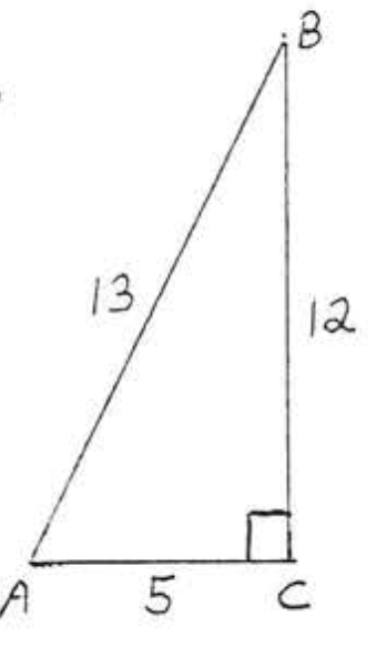
\(\cos A = \dfrac{\text{adj}}{\text{hyp}} = \dfrac{5}{13}\),\(\tan A = \dfrac{\text{opp}}{\text{adj}} = \dfrac{12}{5}\).
Respuesta:\(\cos A = \dfrac{5}{13}\),\(\tan A = \dfrac{12}{5}\).
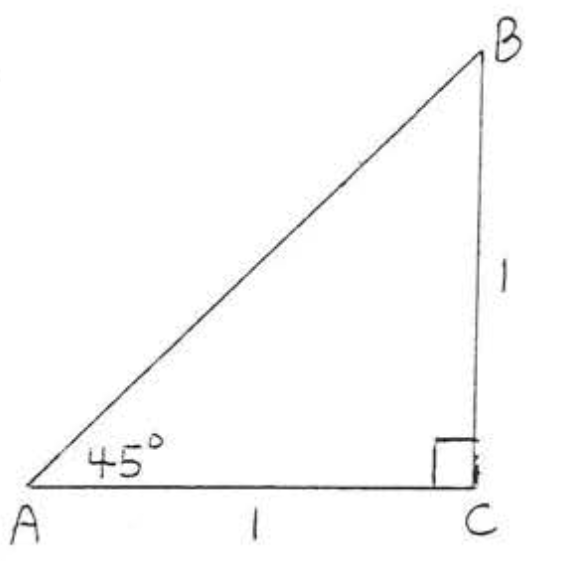
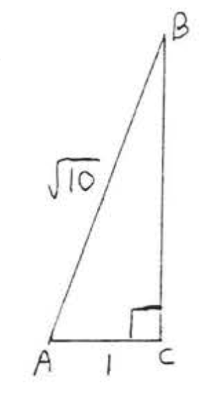
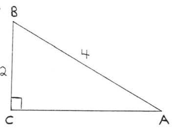
Si\(\tan A = 2\) encuentra\(\sin A\) y\(\cos A\).
Solución
\(\tan A = \dfrac{\text{opp}}{\text{adj}} = 2 = \dfrac{2}{1}\). Dejar\(\triangle ABC\) ser tal que\(a=\) la pierna opuesta\(\angle A = 2\) y\(b =\) la pierna adyacente a\(\angle A = 1\). Ver Figura\(\PageIndex{5}\).
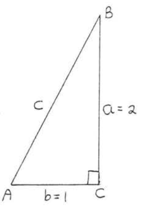
\(\begin{array} {rcl} {a^2 + b^2} & = & {c^2} \\ {2^2 + 1^2} & = & {c^2} \\ {4 + 1} & = & {c^2} \\ {5} & = & {c^2} \\ {\sqrt{5}} & = & {c} \end{array}\)
\(\sin A = \dfrac{\text{opp}}{\text{hyp}} = \dfrac{2}{\sqrt{5}} = \dfrac{2}{\sqrt{5}} \dfrac{\sqrt{5}}{\sqrt{5}} = \dfrac{2\sqrt{5}}{5}\).
\(\cos A = \dfrac{\text{adj}}{\text{hyp}} = \dfrac{1}{\sqrt{5}} = \dfrac{1}{\sqrt{5}} \dfrac{\sqrt{5}}{\sqrt{5}} = \dfrac{\sqrt{5}}{5}\).
Respuesta:\(\sin A = \dfrac{2\sqrt{5}}{5}\),\(\cos A = \dfrac{\sqrt{5}}{5}\).
Problemas
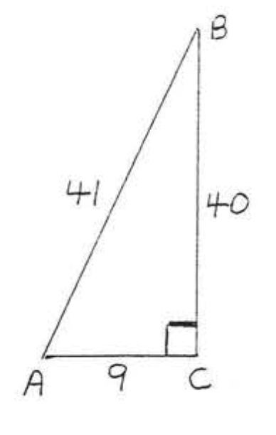
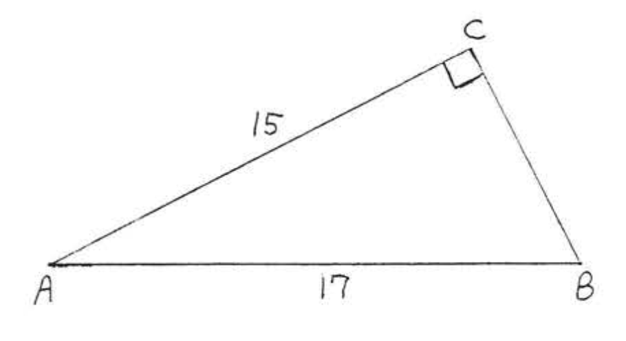
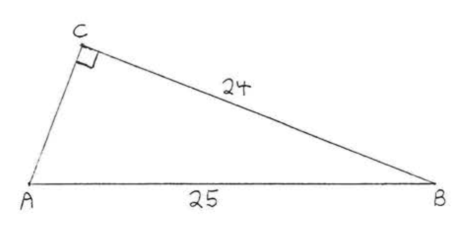
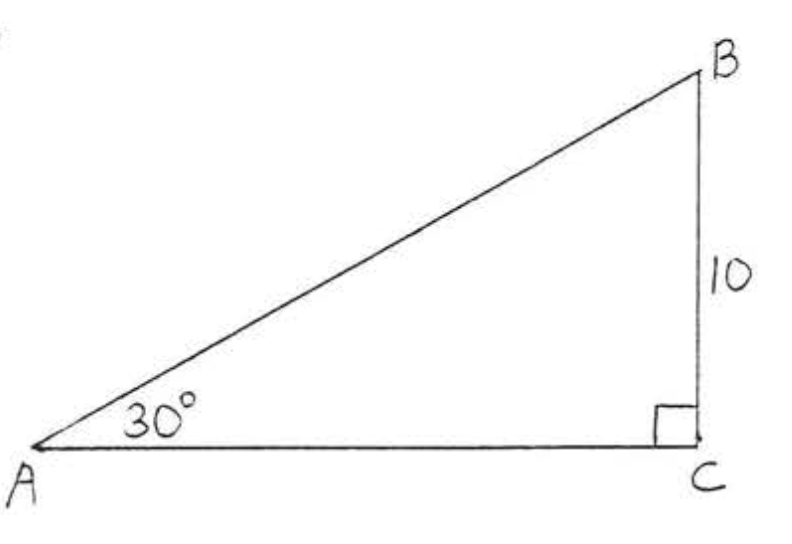
1 - 14. Buscar\(\sin A, \cos A, \tan A, \sin B, \cos B\), y\(\tan B\):
1.
2.
3.
4.
5.
6.
7.
8.
9.
10.
11.
12.
13.
14.
15. Si\(\sin A = \dfrac{4}{5}\) encuentra\(\cos A\) y\(\tan A\).
16. Si\(\sin A = \dfrac{\sqrt{2}}{2}\) encuentra\(\cos A\) y\(\tan A\).
17. Si\(\cos A = \dfrac{\sqrt{3}}{2}\) encuentra\(\sin A\) y\(\tan A\).
18. Si\(\cos A = \dfrac{1}{3}\) encuentra\(\sin A\) y\(\tan A\).
19. Si\(\tan A = 3\) encuentra\(\sin A\) y\(\cos A\).
20. Si\(\tan A = 1\) encuentra\(\sin A\) y\(\cos A\).