
8.2: Soluciones para el Capítulo 2
- Page ID
- 112232

¡El experto tiene razón! La propuesta viola la propiedad (a) cuando x\(_{1}\) = −1, x\(_{2}\) = 0, y\(_{1}\) = −1 e y\(_{2}\) = 1.
De hecho −1 ≤ −1 y 0 ≤ 1, pero −1 ∗ 0 = 0\(\nleq\) −1 = −1 ∗ 1.
Para comprobar que (Disco (M), =, ∗, e) es un preorden monoidal simétrico, necesitamos verificar que nuestros datos propuestos obedecen a las condiciones (a) - (d) de la Definición 2.2. La condición (a) solo establece la tautología que \(_{1}\)x x\(_{2}\) = x\(_{1}\) x\(_{2}\), las condiciones (b) y (c) son precisamente las ecuaciones Eq. (2.7), y (d) es la condición de conmutatividad. Así que ya terminamos. Te dejamos a ti decidir si estábamos diciendo la verdad cuando dijimos que era fácil.
1. Aquí hay una prueba línea por línea, donde escribimos el motivo de cada paso entre paréntesis a la derecha.
Recordemos que llamamos a las propiedades (a) y (c) en la Definición 2.2 monotonicidad y asociatividad respectivamente.
t + u ≤ (v + w) + u (monotonicidad, t ≤ v + w, u ≤ u)
= v + (w + u) (asociatividad)
≤ v + (x + z) (monotonicidad, v ≤ v, w + u ≤ x + v)
= (v + x) + z (asociativicia)
≤ y + z. (monotonicidad, v + x ≤ y, z ≤ z)
- Usamos reflexividad cuando afirmamos que u ≤ u, v ≤ v y z ≤ z, y usamos la transitividad para afirmar que la secuencia de desigualdades anterior implica la desigualdad única t + u ≤ y + z .
- Sabemos que el axioma de simetría no es necesario porque ningún par de cables se cruzan.
La condición (a), monotonicidad, dice que si x → y y z → w son reacciones, entonces x + z → y + w es una reacción. La condición (b), la unidad, se mantiene como 0 representa no tener material, y no agregar material a algún otro material no lo cambia. Condición (c), asociatividad, dice que al combinar tres colecciones x, y y z de moléculas no importa si combinas x e y luego z, o combinas x con y ya combinadas con z. Condición (d), simetría, dice que combinar x con y es lo mismo que combinar y con x. Todo esto es cierto en nuestro modelo de química, por lo que (Mat, →, 0, +) forma un preorden monoidal simétrico.
La unidad monoidal debe ser falsa. El preorden monoidal simétrico satisface el resto de condiciones; esto se puede verificar con solo verificar todos los casos.
La unidad monoidal es el número natural 1. Como sabemos que (\(\mathbb{N}\), ≤) es un preorden, solo necesitamos verificar que ∗ sea monótona, asociativa, unital con 1, y simétrica. Todos estos son hechos familiares de la aritmética.
Esta propuesta no es monótona: tenemos 1|1 y 1|2, sino (1 + 1)\(\not |\) (1 + 2).
1.
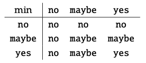
2. Necesitamos mostrar que (a) si x ≤ y y z ≤ w, entonces min (x, z) ≤ min (y, w), (b) min (x, sí) = x = min (sí, x), (c) min (min (x, y), z) = min (x, min (y, z)), y (d) min (x, y) = min (y, z). La forma más sencilla es simplemente verificar todos los casos.
Sí, (P (S), ≤, S,) es un preorden monoidal simétrico.
Dependiendo de tu estado de ánimo, podrías llegar a cualquiera de los siguientes. Primero, podríamos tomar la unidad monoidal como alguna afirmación verdadera que sea cierta para todos los números naturales, como “n es un número natural”.
Podemos emparejar esta unidad con el producto monoidal\(\land\), que toma las declaraciones P y Q y hace la declaración P\(\land\) Q, donde (P\(\land\) Q) (n) es verdadera si P (n) y Q (n) son verdaderas, y falsas de lo contrario. Entonces (Prop\(^{\mathbb{N}}\), ≤, true,\(\land\)) forma un preorden monoidal simétrico.
Otra opción es tomar define false para ser alguna afirmación que sea falsa para todos los números naturales, como “n + 10 ≤ 1” o “n está hecho de queso”.
También podemos definir\(\lor\) tal que (P\(\lor\) Q) (n) es verdadero si y solo si al menos uno de P (n) y Q (n) es verdadero. Entonces (Prop\(^{\mathbb{N}}\), ≤, false,\(\lor\)) forma un preorden monoidal simétrico.
La unitalidad y la asociatividad no tienen nada que ver con el orden en X\(^{op}\): simplemente afirman que I x = x = x I, y (x y) z = x (y z). Ya que estos son ciertos en X, son ciertos en\(^{op}\) X. Simetría es un poco más complicado, ya que en solo pide que x y es equivalente a y x. Sin embargo, esto sigue siendo cierto en X\(^{op}\) porque es cierto en X. De hecho, el hecho de que\(\cong\) (x y) (y x) en X significa que (x y) ≤ (y x) e (y x) ) ≤ (x y) en X, lo que implica respectivamente que (y x) ≤ (x y) y (x y) ≤ (y x) en X\(^{op}\), y por lo tanto que (x y) \(\cong\)(y x) en X\(^{op}\) también.
1. El costo de preorden\(^{op}\) tiene el conjunto subyacente [0, ∞], y el orden creciente habitual en números reales ≤ como su orden.
2. Su unidad monoidal es 0.
3. Su producto monoidal es +.
1. El mapa g es monótona como g (falso) = ∞ ≥ 0 = g (verdadero), satisface la condición (a) ya que 0 ≥ 0 = g (verdadero), y satisface la condición (b) ya que
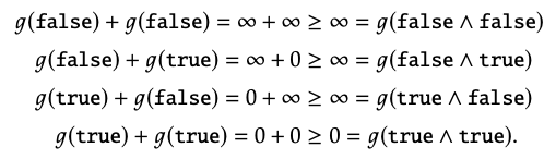
2. Dado que todas las desigualdades con respecto a (a) y (b) anteriores son en realidad igualdades, g es una monótona monoidal estricta.
La respuesta a todas estas preguntas es sí: d y u son ambos monótonos monoidales estrictos. Aquí hay una manera de interpretar esto. La función d pregunta 'es x ��= 0? '. Esto es monótono, 0 es 0, y la suma de dos elementos de [0, ∞] es 0 si y solo si ambos son 0. La función u pregunta '¿es x finita?'. Del mismo modo, esto es monótona, 0 es finita, y la suma de x e y es finita si y solo si x e y son finitas.
- Sí, la multiplicación es monotónica en ≤, unital con respecto a 1, asociativa y simétrica, por lo que (\(\mathbb{N}\), ≤, 1, ∗) es un preorden monoidal. También cumplimos con esta preorden en el Ejercicio 2.31.
- El mapa f (n) = 1 para todos n\(\in\)\(\mathbb{N}\) define una f monótona monoidal: (\(\mathbb{N}\), ≤, 0, +) → (\(\mathbb{N}\), ≤, 1, ∗). (De hecho, ¡es único! ¿Por qué?)
- (\(\mathbb{Z}\), ≤, ∗, 1) no es un preorden monoidal porque ∗ no es monótona. De hecho −1 ≤ 0 pero (−1 ∗ −1)\(\nleq\) (0 ∗ 0).
- Sea (P, ≤) un preorden. ¿Cómo es esto una categoría Bool? Siguiendo el Ejemplo 2.47, podemos construir un Bool -categoría X\(_{P}\) con P como su conjunto de objetos, y con X\(_{P}\) (p, q) := true si p ≤ q, y X\(_{P}\) (p, q) := false de lo contrario. ¿Cómo convertimos esto de nuevo en un preorder? Siguiendo la prueba del Teorema 2.49, construimos un preorden con el conjunto subyacente Ob (X\(_{P}\)) = P, y con p ≤ q si y solo si X\(_{P}\) (p, q) = true. ¡Este es precisamente el preorden (P, ≤)!
- Que X sea una categoría Bool. Por la prueba del Teorema 2.49, construimos un preorden (Ob (X), ≤), donde x ≤ y si y sólo si X (x, y) = true. Entonces, siguiendo nuestra generalización del Ejemplo 2.47 en 1., construimos una Bool -categoría X′ cuyo conjunto de objetos es Ob (X), y tal que X′ (x, y) = true si y solo si x ≤ y in (Ob (X), ≤). Pero por construcción, esto significa X′ (x, y) = X (x, y). Entonces recuperamos la categoría Bool con la que empezamos.
La distancia d (US, España) es mayor: la distancia desde, por ejemplo, San Diego a cualquier lugar es España es mayor que la distancia de cualquier parte de España a la ciudad de Nueva York.
La diferencia entre un espacio métrico Lawvere es decir, una categoría enriquecida sobre ([0, ∞], ≥, 0, +) y una categoría enriquecida sobre (\(\mathbb{R}_{≥0}\), ≥, 0, +) es que en esta última, no se permiten distancias infinitas entre puntos. Por lo tanto, podría llamar a este último un espacio métrico Lawvere de distancia finita.
La tabla de distancias para X es

La matriz de pesos de borde de X es
Un NMY -categoría X es un conjunto X junto con, para todos los pares de elementos x, y en X, un valor X (x, y) igual a no, tal vez, o sí. Además, debemos tener X (x, x) = sí y min (X (x, y), X (y, z)) ≤ X (x, z) para todos x, y, z. Así que una categoría NMY puede ser pensada como un conjunto de puntos junto con una declaración —no, tal vez, o sí— de si es posible llegar de un punto a otro. En particular, siempre es posible llegar a un punto si ya estás ahí, y es lo menos posible llegar de x a z como es llegar de x a y y luego de y a z.
Aquí hay una manera de hacer esta tarea.
1.
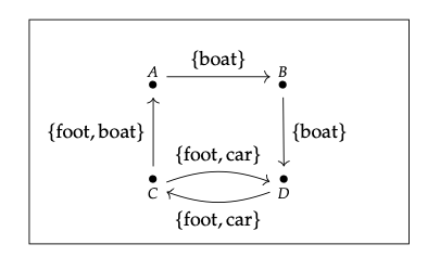
2. La categoría M correspondiente, llámala X, tiene hom-objects:
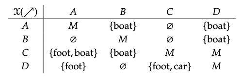
Por ejemplo, para calcular el hom-object X (C, D), notamos que hay dos rutas: C → A → B → D y C → D. Para el primer camino, la intersección es el conjunto {barco}. Para el segundo camino, la intersección en el conjunto {pie, carro}. Su unión, y así el hom-objeto X (C, D), es todo el conjunto M.
Este cálculo contiene la clave de por qué X es una categoría M: al tomar la unión sobre todos los caminos, nos aseguramos de que X (x, y) X (y, z)\(\subseteq\) X (x, z) para todos x, y, z.
3. La interpretación de la persona nos parece correcta.
1.
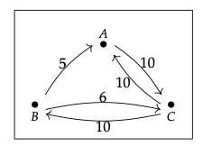
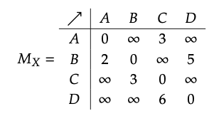
2. La matriz M con (x, y)\(^{th}\) entry equal to the maximum, taken over all paths p from x to y, of the minimum edge label in p is
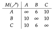
3. This is a matrix of hom-objects for a W-category since the diagonal values are all equal to the monoidal unit ∞, and because min(M(x, y), M(y, z)) ≤ M(x, y) for all x, y, z \(\in\) {A, B, C}.
4. One interpretation is as a weight limit (not to be confused with ‘weighted limit,’ a more advanced categorical notion), for example for trucking cargo between cities. The hom-object indexed by a pair of points (x, y) describes the maximum cargo weight allowed on that route. There is no weight limit on cargo that remains at some point x, so the hom-object from x to x is always infinite. The maximum weight that can be trucked from x to z is always at least the minimum of that that can be trucked from x to y and then y to z. (It is ‘at least’ this much because there may be some other, better route that does not pass through y.)
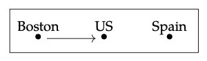
This preorder describes the ‘is a part of’ relation. That is, x ≤ y when d(x, y) = 0, which happens when x is a part of y. So Boston is a part of the US, and Spain is a part of Spain, but the US is not a part of Boston.
1. Recall the monoidal monotones d and u from Exercise 2.44. The function f is equal to d; let g be equal to u.
2. Let X be the Lawvere metric space with two objects A and B, such that d(A, B) = d(B, A) = 5. Then we have X\(_{f}\) = \(\begin{array}{l} A \\\bullet\end{array}\)\(\begin{array}{l} B \\\bullet\end{array}\) while X\(_{g}\) = \(\begin{array}{l} A \\\bullet\end{array}\)\(\begin{array}{l} B \\\bullet\end{array}\).
- An extended metric space is a Lawvere metric space that obeys in addition the properties (b) if d(x, y) = 0 then x = y, and (c) d(x, y) = d(y, x) of Definition 2.51. Let’s consider the dagger condition first. It says that the identity function to the opposite Cost-category is a functor, and so for all x, y we must have d(x, y) ≤ d(y, x). But this means also that d(y, x) ≤ d(x, y), and so d(x, y) = d(y, x). This is exactly property (c). Now let’s consider the skeletality condition. This says that if d(x, y) = 0 and d(y, x) = 0, then x = y. Thus when we have property (c), d(x, y) = d(y, x), this is equivalent to property (b). Thus skeletal dagger Cost-categories are the same as extended metric spaces!
- Recall from Exercise 1.73 that skeletal dagger preorders are sets. The analogy “preorders are to sets as Lawvere metric spaces are to extended metric spaces” is thus the observation that just as extended metric spaces are skeletal dagger Cost-categories, sets are skeletal dagger Bool- categories.
1. Let (x, y) \(\in\) X × Y. Since X and Y are V-categories, we have I ≤ X(x, x) and I ≤ Y(y, y). Thus I = I ⊗ I ≤ X(x, x) ⊗ Y(y, y) = (X × Y)((x, y), (x, y)).
2. Using the definition of product hom-objects, and the symmetry and monotonicity of ⊗ we have
(X × Y)((x\(_{1}\), y\(_{1}\)), (x\(_{2}\), y\(_{2}\))) ⊗ (X × Y)((x\(_{2}\), y\(_{2}\)), (x\(_{3}\), y\(_{3}\)))
= X(x\(_{1}\), x\(_{2}\)) ⊗ Y(y\(_{1}\), y\(_{2}\)) ⊗ X(x\(_{2}\), x\(_{3}\)) ⊗ Y(y\(_{2}\), y\(_{3}\))
= X(x\(_{1}\), x\(_{2}\)) ⊗ X(x\(_{2}\), x\(_{3}\)) ⊗ Y(y\(_{1}\), y\(_{2}\)) ⊗ Y(y\(_{2}\), y\(_{3}\))
≤ X(x\(_{1}\), x\(_{3}\)) ⊗ Y(y\(_{1}\), y\(_{3}\))
= (X × Y)((x\(_{1}\), y\(_{1}\)), (x\(_{3}\), y\(_{3}\))) .
3. In particular, we use the symmetry, to conclude that Y(y\(_{1}\), y\(_{2}\)) ⊗ X(x\(_{2}\), x\(_{3}\)) = X(x\(_{2}\), x\(_{3}\)) ⊗ Y(y\(_{1}\), y\(_{2}\)).
We just apply Definition 2.74(ii): (\(\mathbb{R}\) × \(\mathbb{R}\))((5, 6), (−1, 4)) = \(\mathbb{R}\)(5, −1) + \(\mathbb{R}\)(6, 4) = 6 + 2 = 8.
1. The function−⊗v :V → V is monotone, because if u ≤ u′ then u ⊗ v ≤ u′ ⊗ v by the monotonicity condition (a) in Definition 2.2.
2. Let a := (v -o w) in Eq.(2.80). The right hand side is thus (v -o w) ≤ (v -o w), which is true by reflexivity. Thus the left hand side is true too. This gives ((v -o w) ⊗ v) ≤ w.
3. Let u ≤ u′. Then, using 2., (v -o u) ⊗ v ≤ u ≤ u′. Applying Eq.(2.80), we thus have (v -o u) ≤ (v -o u′). This shows that the map (v -o −): V → V is monotone.
4. Eq.(2.80) is exactly the adjointness condition from Definition 1.95, except for the fact that we do not know (− ⊗ v) and (v -o −) are monotone maps. We proved this, however, in items 1 and 3 above.
We need to find the hom-element. This is given by implication. That is, define the function x ⇒ y by the table
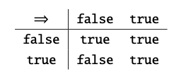
Then (a \(\land\) v) ≤ w if and only if a ≤ (v ⇒ w). Indeed, if v = false then a \(\land\) false = false, and so the left hand side is always true.
But (false ⇒ w) = true, so the right hand side is always true too. If v = true, then a \(\land\) true = a so the left hand side says a ≤ w.
But (true ⇒ w) = w, so the right hand side is the same. Thus ⇒ defines a hom-element as per Eq. (2.80).
We showed in Exercise 2.84 that Bool is symmetric monoidal closed, and in Exercise 1.7 and Example 1.88 that the join is given by the OR operation \(\lor\). Thus Bool is a quantale.
Yes, the powerset monoidal preorder (P(S), \(\subseteq\), S, ∩) is a quantale. The hom-object B -o C is given by \(\bar{B}\) \(\bigcup\) C, where \(\bar{B}\) is the complement of B: it contains all elements of S not contained in B.
To see that this satisfies Eq. (2.80), note that if (A ∩ B) \(\subseteq\) C, then
A = (A ∩ \(\bar{B}\)) \(\bigcup\) (A ∩ B) \(\subseteq\) \(\bar{B}\) \(\bigcup\) C.
On the other hand, if A \(\subseteq\) (\(\bar{B}\) \(\bigcup\) C), then
A ∩ B \(\subseteq\) (\(\bar{B}\) \(\bigcup\) C) ∩ B (\(\bar{B}\) ∩ B) \(\bigcup\) (C ∩ B) = C ∩ B \(\subseteq\) C.
So (P(S), \(\subseteq\), S, ∩) is monoidal closed. Furthermore, joins are given by union of subobjects, so it is a quantale.
1a. In Bool, (\(\bigvee\) Ø) = false, the least element.
1b. In Cost, (\(\bigvee\) Ø) = ∞. This is because we use the opposite order ≥ on [0, ∞], so \(\bigvee\) Ø is the greatest element of [0, ∞]. Note that in this case our convention from Definition 2.90, where we denote (\(\bigvee\) Ø) = 0, is a bit confusing! Beware!
2a. In Bool, x (\lor\) y is the usual join, OR.
2b. In Cost, x (\lor\) y is the minimum min(x, y). Again because we use the opposite order on [0, ∞], the join is the greatest number less than or equal to x and y.
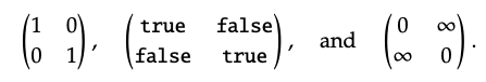
The 2 × 2-identity matrices for (\(\mathbb{N}\), ≤, 1, ∗), Bool, and Cost are respectively
1. We first use Proposition 2.87 (2) and symmetry to show that for all v \(\in\) V, 0 ⊗ v = 0.
0 ⊗ v \(\cong\) v ⊗ 0 \(\cong\) (v ⊗ \(\bigvee_{a \in Ø}\)a) = \(\bigvee_{a \in Ø}\)(v ⊗ a) = 0.
Then we may just follow the definition in Eq. (2.101):
\(\begin{aligned}
I_{X} * M(x, y) &=\bigvee_{x^{\prime} \in X} I_{X}\left(x, x^{\prime}\right) \otimes M\left(x^{\prime}, y\right) \\
&=\left(I_{X}(x, x) \otimes M(x, y)\right) \vee\left(\bigvee_{x^{\prime} \in X, x^{\prime} \neq x} I_{X}\left(x, x^{\prime}\right) \otimes M\left(x^{\prime}, y\right)\right) \\
&=(I \otimes M(x, y)) \vee\left(\bigvee_{x^{\prime} \in X, x^{\prime} \neq x} 0 \otimes M\left(x^{\prime}, y\right)\right) \\
&=M(x, y) \vee 0=M(x, y) .
\end{aligned}\)
2. This again follows from Proposition 2.87(2) and symmetry, making use also of the associativity of ⊗:
\(\begin{aligned}
((M * N) * P)(w, z) &=\bigvee_{y \in Y}\left(\bigvee_{x \in X} M(w, x) \otimes N(x, y)\right) \otimes P(y, z) \\
& \cong \bigvee_{y \in Y, x \in X} M(w, x) \otimes N(x, y) \otimes P(y, z) \\
& \cong \bigvee_{x \in X} M(w, x) \otimes\left(\bigvee_{y \in Y} N(x, y) \otimes P(y, z)\right) \\
&=(M *(N * P))(w, z)
\end{aligned}\)
We have the matrices