8.3: Aritmética mental: uso de la propiedad distributiva

Última actualización
Guardar como PDF

Page ID: 116443

$ \newcommand{\vecs}[1]{\overset { \scriptstyle \rightharpoonup} {\mathbf{#1}} } $

$ \newcommand{\vecd}[1]{\overset{-\!-\!\rightharpoonup}{\vphantom{a}\smash {#1}}} $

$ \newcommand{\id}{\mathrm{id}}$ $ \newcommand{\Span}{\mathrm{span}}$

( \newcommand{\kernel}{\mathrm{null}\,}\) $ \newcommand{\range}{\mathrm{range}\,}$

$ \newcommand{\RealPart}{\mathrm{Re}}$ $ \newcommand{\ImaginaryPart}{\mathrm{Im}}$

$ \newcommand{\Argument}{\mathrm{Arg}}$ $ \newcommand{\norm}[1]{\| #1 \|}$

$ \newcommand{\inner}[2]{\langle #1, #2 \rangle}$

$ \newcommand{\Span}{\mathrm{span}}$

$ \newcommand{\id}{\mathrm{id}}$

$ \newcommand{\Span}{\mathrm{span}}$

$ \newcommand{\kernel}{\mathrm{null}\,}$

$ \newcommand{\range}{\mathrm{range}\,}$

$ \newcommand{\RealPart}{\mathrm{Re}}$

$ \newcommand{\ImaginaryPart}{\mathrm{Im}}$

$ \newcommand{\Argument}{\mathrm{Arg}}$

$ \newcommand{\norm}[1]{\| #1 \|}$

$ \newcommand{\inner}[2]{\langle #1, #2 \rangle}$

$ \newcommand{\Span}{\mathrm{span}}$ $ \newcommand{\AA}{\unicode[.8,0]{x212B}}$

$ \newcommand{\vectorA}[1]{\vec{#1}} % arrow$

$ \newcommand{\vectorAt}[1]{\vec{\text{#1}}} % arrow$

$ \newcommand{\vectorB}[1]{\overset { \scriptstyle \rightharpoonup} {\mathbf{#1}} } $

$ \newcommand{\vectorC}[1]{\textbf{#1}} $

$ \newcommand{\vectorD}[1]{\overrightarrow{#1}} $

$ \newcommand{\vectorDt}[1]{\overrightarrow{\text{#1}}} $

$ \newcommand{\vectE}[1]{\overset{-\!-\!\rightharpoonup}{\vphantom{a}\smash{\mathbf {#1}}}} $

$ \newcommand{\vecs}[1]{\overset { \scriptstyle \rightharpoonup} {\mathbf{#1}} } $

$ \newcommand{\vecd}[1]{\overset{-\!-\!\rightharpoonup}{\vphantom{a}\smash {#1}}} $

$\newcommand{\avec}{\mathbf a}$ $\newcommand{\bvec}{\mathbf b}$ $\newcommand{\cvec}{\mathbf c}$ $\newcommand{\dvec}{\mathbf d}$ $\newcommand{\dtil}{\widetilde{\mathbf d}}$ $\newcommand{\evec}{\mathbf e}$ $\newcommand{\fvec}{\mathbf f}$ $\newcommand{\nvec}{\mathbf n}$ $\newcommand{\pvec}{\mathbf p}$ $\newcommand{\qvec}{\mathbf q}$ $\newcommand{\svec}{\mathbf s}$ $\newcommand{\tvec}{\mathbf t}$ $\newcommand{\uvec}{\mathbf u}$ $\newcommand{\vvec}{\mathbf v}$ $\newcommand{\wvec}{\mathbf w}$ $\newcommand{\xvec}{\mathbf x}$ $\newcommand{\yvec}{\mathbf y}$ $\newcommand{\zvec}{\mathbf z}$ $\newcommand{\rvec}{\mathbf r}$ $\newcommand{\mvec}{\mathbf m}$ $\newcommand{\zerovec}{\mathbf 0}$ $\newcommand{\onevec}{\mathbf 1}$ $\newcommand{\real}{\mathbb R}$ $\newcommand{\twovec}[2]{\left[\begin{array}{r}#1 \\ #2 \end{array}\right]}$ $\newcommand{\ctwovec}[2]{\left[\begin{array}{c}#1 \\ #2 \end{array}\right]}$ $\newcommand{\threevec}[3]{\left[\begin{array}{r}#1 \\ #2 \\ #3 \end{array}\right]}$ $\newcommand{\cthreevec}[3]{\left[\begin{array}{c}#1 \\ #2 \\ #3 \end{array}\right]}$ $\newcommand{\fourvec}[4]{\left[\begin{array}{r}#1 \\ #2 \\ #3 \\ #4 \end{array}\right]}$ $\newcommand{\cfourvec}[4]{\left[\begin{array}{c}#1 \\ #2 \\ #3 \\ #4 \end{array}\right]}$ $\newcommand{\fivevec}[5]{\left[\begin{array}{r}#1 \\ #2 \\ #3 \\ #4 \\ #5 \\ \end{array}\right]}$ $\newcommand{\cfivevec}[5]{\left[\begin{array}{c}#1 \\ #2 \\ #3 \\ #4 \\ #5 \\ \end{array}\right]}$ $\newcommand{\mattwo}[4]{\left[\begin{array}{rr}#1 \amp #2 \\ #3 \amp #4 \\ \end{array}\right]}$ $\newcommand{\laspan}[1]{\text{Span}\{#1\}}$ $\newcommand{\bcal}{\cal B}$ $\newcommand{\ccal}{\cal C}$ $\newcommand{\scal}{\cal S}$ $\newcommand{\wcal}{\cal W}$ $\newcommand{\ecal}{\cal E}$ $\newcommand{\coords}[2]{\left\{#1\right\}_{#2}}$ $\newcommand{\gray}[1]{\color{gray}{#1}}$ $\newcommand{\lgray}[1]{\color{lightgray}{#1}}$ $\newcommand{\rank}{\operatorname{rank}}$ $\newcommand{\row}{\text{Row}}$ $\newcommand{\col}{\text{Col}}$ $\renewcommand{\row}{\text{Row}}$ $\newcommand{\nul}{\text{Nul}}$ $\newcommand{\var}{\text{Var}}$ $\newcommand{\corr}{\text{corr}}$ $\newcommand{\len}[1]{\left|#1\right|}$ $\newcommand{\bbar}{\overline{\bvec}}$ $\newcommand{\bhat}{\widehat{\bvec}}$ $\newcommand{\bperp}{\bvec^\perp}$ $\newcommand{\xhat}{\widehat{\xvec}}$ $\newcommand{\vhat}{\widehat{\vvec}}$ $\newcommand{\uhat}{\widehat{\uvec}}$ $\newcommand{\what}{\widehat{\wvec}}$ $\newcommand{\Sighat}{\widehat{\Sigma}}$ $\newcommand{\lt}{<}$ $\newcommand{\gt}{>}$ $\newcommand{\amp}{&}$ $\definecolor{fillinmathshade}{gray}{0.9}$

Objetivos de aprendizaje

entender la propiedad distributiva
ser capaz de obtener el resultado exacto de una multiplicación usando la propiedad distributiva

La propiedad distributiva

Propiedad distributiva
La propiedad distributiva es una característica de los números que implica tanto la suma como la multiplicación. Se usa a menudo en álgebra, y podemos usarlo ahora para obtener resultados exactos para una multiplicación.

Supongamos que deseamos calcular$3(2 + 5)$. Podemos proceder de cualquiera de dos maneras, una manera que ya conocemos (el orden de las operaciones), y una nueva vía (la propiedad distributiva).

Calcular$3(2 + 5)$ usando el orden de las operaciones.
$3(2 + 5)$
Operar primero dentro de los paréntesis:$2 + 5 = 7$.
$3(2 + 5) = 3 \cdot 7$
Ahora multiplica 3 y 7.
$3(2 + 5) = 3 \cdot 7 = 21$
Así,$3(2 + 5) = 21$.
Calcular$3(2 + 5)$ usando la propiedad de distribución.
Sabemos que la multiplicación describe la adición repetida. Así,
$\begin{array} {rclc} {3(2 + 5)} & = & {\underbrace{2 + 5 + 2 + 5 + 2 + 5}_{\text{2 + 5 appears 3 times}}} & {} \\ {} & = & {2 + 2 + 2 + 5 + 5 + 5} & {\text{(by the commutative property of addition)}} \\ {} & = & {3 \cdot 2 + 3 \cdot 5} & {\text{(since multiplication describes repeated addition)}} \\ {} & = & {6 + 15} & {} \\ {} & = & {21} & {} \end{array}$
Así,$3(2 + 5) = 21$.
Veamos de nuevo este uso de la propiedad distributiva.
$3(2 + 5) = \underbrace{2 + 5 + 2 + 5 + 2 + 5}_{2 + 5 appears 3 times}$
$3(2 + 5) = \underbrace{2 + 2 + 2}_{2 appears 3 times} + \underbrace{5 + 5 + 5}_{5 appears 3 times}$
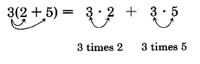
$3 veces la cantidad dos más cinco. Las flechas apuntan desde los tres hasta los dos y los cinco. Esto es igual a tres por dos más tres por cinco.$
El 3 ha sido distribuido a los 2 y 5.

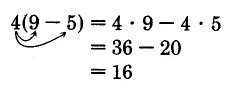
Esta es la propiedad distributiva. Distribuimos el factor a cada adenda entre paréntesis. La propiedad distributiva funciona tanto para sumas como para diferencias.

Conjunto de Muestras A

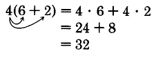
$4 veces la cantidad 6 más 2. Las flechas apuntan desde el 4 hasta tanto el 6 como el 2. Esto es igual a 4 veces 6 más 4 veces 2. Esto es igual a 24 más 8, que es igual a 32.$

Usando el orden de operaciones, obtenemos

$\begin{array} {rcl} {4(6 + 2)} & = & {4 \cdot 8} \\ {} & = & {32} \end{array}$

Conjunto de Muestras A

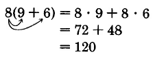
$8 veces la cantidad 9 más 6. Las flechas apuntan desde el 8 hasta el 9 y el 6. Esto es igual a 8 veces 9 más 8 veces 6. Esto es igual a 72 más 48, que es igual a 120.$

Usando el orden de operaciones, obtenemos

$\begin{array} {rcl} {8(9 + 6)} & = & {8 \cdot 15} \\ {} & = & {120} \end{array}$

Conjunto de Muestras A

$4 veces la cantidad 9 menos 5. Las flechas apuntan desde el 4 hasta tanto el 9 como el 5. Esto es igual a 4 veces 9 menos 4 veces 5. Esto es igual a 36 menos 20, que es igual a 16.$

Conjunto de Muestras A

$25 veces la cantidad 20 menos 3. Las flechas apuntan desde el 20 hasta tanto el 20 como el 3. Esto es igual a 25 veces 20 menos 25 veces 3. Esto es igual a 500 menos 76, que es igual a 425.$

Conjunto de práctica A

Utilice la propiedad distributiva para calcular cada valor.

$6(8 + 4)$

Contestar: $6 \cdot 8 + 6 \cdot 4 = 48 + 24 = 72$

Conjunto de práctica A

$4(4 + 7)$

Contestar: $4 \cdot 4 + 4 \cdot 7 = 16 + 28 = 44$

Conjunto de práctica A

$8(2 + 9)$

Contestar: $8 \cdot 2 + 8 \cdot 9 = 16 + 72 = 88$

Conjunto de práctica A

$12(10 + 3)$

Contestar: $12 \cdot 10 + 12 \cdot 3 = 120 + 36 = 156$

Conjunto de práctica A

$6(11 - 3)$

Contestar: $6 \cdot 11 - 6 \cdot 3 = 66 - 18 = 48$

Conjunto de práctica A

$8(9 - 7)$

Contestar: $8 \cdot 9 - 8 \cdot 7 = 72 - 56 = 16$

Conjunto de práctica A

$15(30 - 8)$

Contestar: $15 \cdot 30 - 15 \cdot 8 = 450 - 120 = 330$

Estimación usando la propiedad distributiva

Podemos utilizar la propiedad distributiva para obtener resultados exactos para productos como$25 \cdot 23$. La propiedad distributiva funciona mejor para productos cuando uno de los factores termina en 0 o 5. Restringiremos nuestra atención únicamente a dichos productos.

Conjunto de Muestras B

Utilice la propiedad distributiva para calcular cada valor.

$25 \cdot 23$

Solución

Observe eso$23 = 20 + 3$. Ahora escribimos

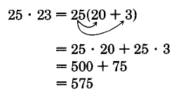
$25 veces 23 equivale a 25 veces la cantidad 20 más 3. Esto es igual a 25 veces 20 más 25 veces 3. Esto es igual a 500 + 75. Esto es igual a 575.$

Por lo tanto,$25 \cdot 23 = 575$

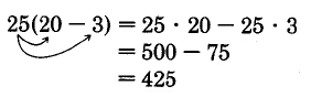
Podríamos haber procedido escribiendo 23 como$30 - 7$.

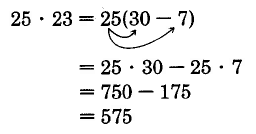
$25 veces 23 equivale a 25 veces la cantidad 30 menos 7. Esto es igual a 25 veces 30 menos 25 veces 7. Esto es igual a 750 menos 175. Esto es igual a 575.$

Conjunto de Muestras B

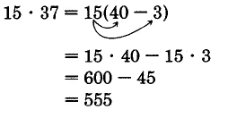
$15 \cdot 37$

Solución

Observe eso$37 = 30 + 7$. Ahora escribimos

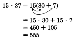
$15 veces 37 equivale a 15 veces la cantidad 30 más 7. Esto es igual a 15 veces 30 más 15 veces 7. Esto es igual a 450 más 105, que es igual a 555.$

Por lo tanto,$15 \cdot 37 = 555$

Podríamos haber procedido escribiendo 37 como$40 - 3$.

$15 veces 37 equivale a 15 veces la cantidad 40 menos 3. Esto es igual a 15 veces 40 más 15 veces 3. Esto es igual a 600 menos 45, que es igual a 555.$

Conjunto de Muestras B

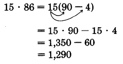
$15 \cdot 86$

Solución

Observe eso$86 = 80 + 6$. Ahora escribimos

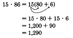
$15 veces 86 equivale a 15 veces la cantidad 80 más 6. Esto es igual a 15 veces 80 más 15 veces 6. Esto equivale a 1,200 más 90, lo que equivale a 1,290.$

Podríamos haber procedido escribiendo 86 como$90 - 4$.

$15 veces 86 equivale a 15 veces la cantidad 90 menos 4. Esto es igual a 15 veces 90 menos 15 veces 4. Esto es igual a 1,350 menos 60, que es igual a 1,290.$

Set de práctica B

Utilice la propiedad distributiva para calcular cada valor.

$25 \cdot 12$

Contestar: $25(10 + 2) = 25 \cdot 10 + 25 \cdot 2 = 250 + 50 = 300$

Set de práctica B

$35 \cdot 14$

Contestar: $35(10 + 4) = 35 \cdot 10 + 35 \cdot 4 = 350 + 140 = 490$

Set de práctica B

$80 \cdot 58$

Contestar: $80(50 + 8) = 80 \cdot 50 + 80 \cdot 8 = 4,000 + 640 = 4,640$

Set de práctica B

$65 \cdot 62$

Contestar: $65(60 + 2) = 65 \cdot 60 + 65 \cdot 2 = 3,900 + 130 = 4,030$

Ejercicios

Utilice la propiedad distributiva para calcular cada producto.

Ejercicio$\PageIndex{1}$

$15 \cdot 13$

Contestar: $15 (10 + 3) = 150 + 45 = 195$

Ejercicio$\PageIndex{2}$

$15 \cdot 14$

Ejercicio$\PageIndex{3}$

$25 \cdot 11$

Contestar: $25 (10 + 1) = 250 + 25 = 275$

Ejercicio$\PageIndex{4}$

$25 \cdot 16$

Ejercicio$\PageIndex{5}$

$15 \cdot 16$

Contestar: $15 (20 - 4) = 300 - 60 = 240$

Ejercicio$\PageIndex{6}$

$35 \cdot 12$

Ejercicio$\PageIndex{7}$

$45 \cdot 83$

Contestar: $45 (80 + 3) = 3600 + 135 = 3735$

Ejercicio$\PageIndex{8}$

$45 \cdot 38$

Ejercicio$\PageIndex{9}$

$25 \cdot 38$

Contestar: $25 (40 - 2) = 1,000 - 50 = 950$

Ejercicio$\PageIndex{10}$

$25 \cdot 96$

Ejercicio$\PageIndex{11}$

$75 \cdot 14$

Contestar: $75 (10 + 4) = 750 + 300 = 1,050$

Ejercicio$\PageIndex{12}$

$85 \cdot 34$

Ejercicio$\PageIndex{13}$

$65 \cdot 26$

Contestar: $65 (20 + 6) = 1,300 + 390 = 1,690$o$65(30 - 4) = 1,950 - 260 = 1,690$

Ejercicio$\PageIndex{14}$

$55 \cdot 51$

Ejercicio$\PageIndex{15}$

$15 \cdot 107$

Contestar: $15 (100 + 7) = 1,500 + 105 = 1,605$

Ejercicio$\PageIndex{16}$

$25 \cdot 208$

Ejercicio$\PageIndex{17}$

$35 \cdot 402$

Contestar: $35 (400 + 2) = 14,000 + 70 = 14,070$

Ejercicio$\PageIndex{18}$

$85 \cdot 110$

Ejercicio$\PageIndex{19}$

$95 \cdot 12$

Contestar: $95 (10 + 2) = 950 + 190 = 1,140$

Ejercicio$\PageIndex{20}$

$65 \cdot 40$

Ejercicio$\PageIndex{21}$

$80 \cdot 32$

Contestar: $80 (30 + 2) = 2,400 + 160 = 2,560$

Ejercicio$\PageIndex{22}$

$30 \cdot 47$

Ejercicio$\PageIndex{23}$

$50 \cdot 63$

Contestar: $50 (60 + 3) = 3,000 + 150 = 3,150$

Ejercicio$\PageIndex{24}$

$90 \cdot 78$

Ejercicio$\PageIndex{25}$

$40 \cdot 89$

Contestar: $40 (90 - 1) = 3,600 - 40 = 3,560$

Ejercicios para la revisión

Ejercicio$\PageIndex{26}$

Encuentra el mayor factor común de 360 y 3,780.

Ejercicio$\PageIndex{27}$

Reducir$\dfrac{594}{5,148}$ a los términos más bajos.

Contestar: $\dfrac{3}{26}$

Ejercicio$\PageIndex{28}$

$1\dfrac{5}{9}$de$2 \dfrac{4}{7}$ es ¿qué número?

Ejercicio$\PageIndex{29}$

Resuelve la proporción:$\dfrac{7}{15} = \dfrac{x}{90}$

Contestar: $x = 42$

Ejercicio$\PageIndex{30}$

Utilice el método de agrupación para estimar la suma:$88 + 106 + 91 + 114$.

Search

Text Color

Text Size

Margin Size

Font Type