3.2: Transformaciones de Gráficas Comunes

Última actualización
Guardar como PDF

Page ID: 115917

$ \newcommand{\vecs}[1]{\overset { \scriptstyle \rightharpoonup} {\mathbf{#1}} } $

$ \newcommand{\vecd}[1]{\overset{-\!-\!\rightharpoonup}{\vphantom{a}\smash {#1}}} $

$ \newcommand{\id}{\mathrm{id}}$ $ \newcommand{\Span}{\mathrm{span}}$

( \newcommand{\kernel}{\mathrm{null}\,}\) $ \newcommand{\range}{\mathrm{range}\,}$

$ \newcommand{\RealPart}{\mathrm{Re}}$ $ \newcommand{\ImaginaryPart}{\mathrm{Im}}$

$ \newcommand{\Argument}{\mathrm{Arg}}$ $ \newcommand{\norm}[1]{\| #1 \|}$

$ \newcommand{\inner}[2]{\langle #1, #2 \rangle}$

$ \newcommand{\Span}{\mathrm{span}}$

$ \newcommand{\id}{\mathrm{id}}$

$ \newcommand{\Span}{\mathrm{span}}$

$ \newcommand{\kernel}{\mathrm{null}\,}$

$ \newcommand{\range}{\mathrm{range}\,}$

$ \newcommand{\RealPart}{\mathrm{Re}}$

$ \newcommand{\ImaginaryPart}{\mathrm{Im}}$

$ \newcommand{\Argument}{\mathrm{Arg}}$

$ \newcommand{\norm}[1]{\| #1 \|}$

$ \newcommand{\inner}[2]{\langle #1, #2 \rangle}$

$ \newcommand{\Span}{\mathrm{span}}$ $ \newcommand{\AA}{\unicode[.8,0]{x212B}}$

$ \newcommand{\vectorA}[1]{\vec{#1}} % arrow$

$ \newcommand{\vectorAt}[1]{\vec{\text{#1}}} % arrow$

$ \newcommand{\vectorB}[1]{\overset { \scriptstyle \rightharpoonup} {\mathbf{#1}} } $

$ \newcommand{\vectorC}[1]{\textbf{#1}} $

$ \newcommand{\vectorD}[1]{\overrightarrow{#1}} $

$ \newcommand{\vectorDt}[1]{\overrightarrow{\text{#1}}} $

$ \newcommand{\vectE}[1]{\overset{-\!-\!\rightharpoonup}{\vphantom{a}\smash{\mathbf {#1}}}} $

$ \newcommand{\vecs}[1]{\overset { \scriptstyle \rightharpoonup} {\mathbf{#1}} } $

$ \newcommand{\vecd}[1]{\overset{-\!-\!\rightharpoonup}{\vphantom{a}\smash {#1}}} $

$\newcommand{\avec}{\mathbf a}$ $\newcommand{\bvec}{\mathbf b}$ $\newcommand{\cvec}{\mathbf c}$ $\newcommand{\dvec}{\mathbf d}$ $\newcommand{\dtil}{\widetilde{\mathbf d}}$ $\newcommand{\evec}{\mathbf e}$ $\newcommand{\fvec}{\mathbf f}$ $\newcommand{\nvec}{\mathbf n}$ $\newcommand{\pvec}{\mathbf p}$ $\newcommand{\qvec}{\mathbf q}$ $\newcommand{\svec}{\mathbf s}$ $\newcommand{\tvec}{\mathbf t}$ $\newcommand{\uvec}{\mathbf u}$ $\newcommand{\vvec}{\mathbf v}$ $\newcommand{\wvec}{\mathbf w}$ $\newcommand{\xvec}{\mathbf x}$ $\newcommand{\yvec}{\mathbf y}$ $\newcommand{\zvec}{\mathbf z}$ $\newcommand{\rvec}{\mathbf r}$ $\newcommand{\mvec}{\mathbf m}$ $\newcommand{\zerovec}{\mathbf 0}$ $\newcommand{\onevec}{\mathbf 1}$ $\newcommand{\real}{\mathbb R}$ $\newcommand{\twovec}[2]{\left[\begin{array}{r}#1 \\ #2 \end{array}\right]}$ $\newcommand{\ctwovec}[2]{\left[\begin{array}{c}#1 \\ #2 \end{array}\right]}$ $\newcommand{\threevec}[3]{\left[\begin{array}{r}#1 \\ #2 \\ #3 \end{array}\right]}$ $\newcommand{\cthreevec}[3]{\left[\begin{array}{c}#1 \\ #2 \\ #3 \end{array}\right]}$ $\newcommand{\fourvec}[4]{\left[\begin{array}{r}#1 \\ #2 \\ #3 \\ #4 \end{array}\right]}$ $\newcommand{\cfourvec}[4]{\left[\begin{array}{c}#1 \\ #2 \\ #3 \\ #4 \end{array}\right]}$ $\newcommand{\fivevec}[5]{\left[\begin{array}{r}#1 \\ #2 \\ #3 \\ #4 \\ #5 \\ \end{array}\right]}$ $\newcommand{\cfivevec}[5]{\left[\begin{array}{c}#1 \\ #2 \\ #3 \\ #4 \\ #5 \\ \end{array}\right]}$ $\newcommand{\mattwo}[4]{\left[\begin{array}{rr}#1 \amp #2 \\ #3 \amp #4 \\ \end{array}\right]}$ $\newcommand{\laspan}[1]{\text{Span}\{#1\}}$ $\newcommand{\bcal}{\cal B}$ $\newcommand{\ccal}{\cal C}$ $\newcommand{\scal}{\cal S}$ $\newcommand{\wcal}{\cal W}$ $\newcommand{\ecal}{\cal E}$ $\newcommand{\coords}[2]{\left\{#1\right\}_{#2}}$ $\newcommand{\gray}[1]{\color{gray}{#1}}$ $\newcommand{\lgray}[1]{\color{lightgray}{#1}}$ $\newcommand{\rank}{\operatorname{rank}}$ $\newcommand{\row}{\text{Row}}$ $\newcommand{\col}{\text{Col}}$ $\renewcommand{\row}{\text{Row}}$ $\newcommand{\nul}{\text{Nul}}$ $\newcommand{\var}{\text{Var}}$ $\newcommand{\corr}{\text{corr}}$ $\newcommand{\len}[1]{\left|#1\right|}$ $\newcommand{\bbar}{\overline{\bvec}}$ $\newcommand{\bhat}{\widehat{\bvec}}$ $\newcommand{\bperp}{\bvec^\perp}$ $\newcommand{\xhat}{\widehat{\xvec}}$ $\newcommand{\vhat}{\widehat{\vvec}}$ $\newcommand{\uhat}{\widehat{\uvec}}$ $\newcommand{\what}{\widehat{\wvec}}$ $\newcommand{\Sighat}{\widehat{\Sigma}}$ $\newcommand{\lt}{<}$ $\newcommand{\gt}{>}$ $\newcommand{\amp}{&}$ $\definecolor{fillinmathshade}{gray}{0.9}$

La transformación de las gráficas, utilizando funciones comunes, será una habilidad que aportará una visión para graficar funciones de forma rápida y sin dolor. Anticipar cómo se verá una gráfica de una función, y transformar gráficas antiguas en nuevas gráficas, es una habilidad que exploraremos en esta sección. Dominar esta habilidad te dará una ventaja sobre la comprensión de la geometría analítica, un componente clave para el cálculo.

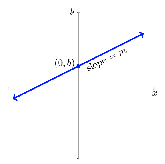
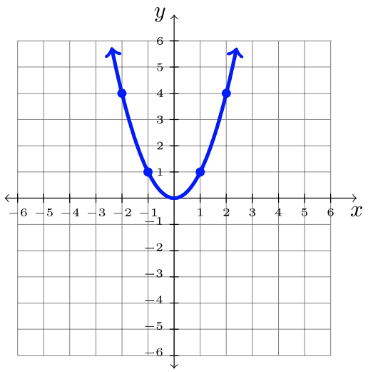
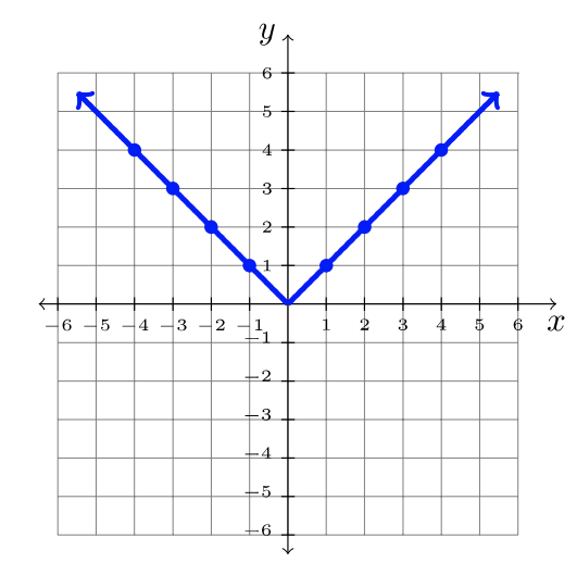
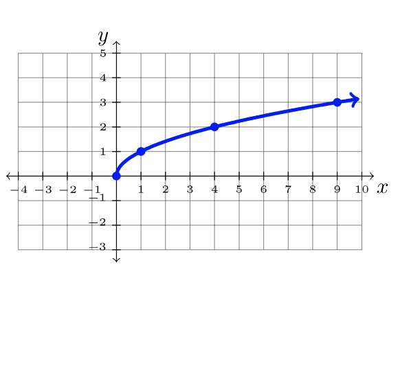
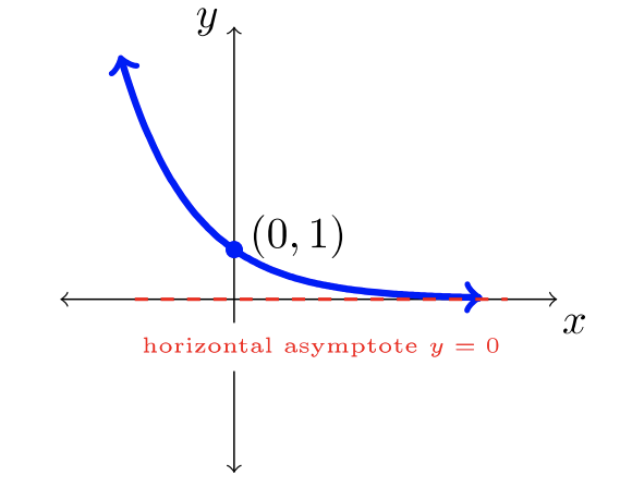
Aquí hay nueve funciones comunes y sus gráficas. Cada una de estas funciones se denominará “la función padre” por su familia de funciones transformadas.

$f(x) = mx + b$	$f(x) = x^2$	$f(x) = \|x\|$
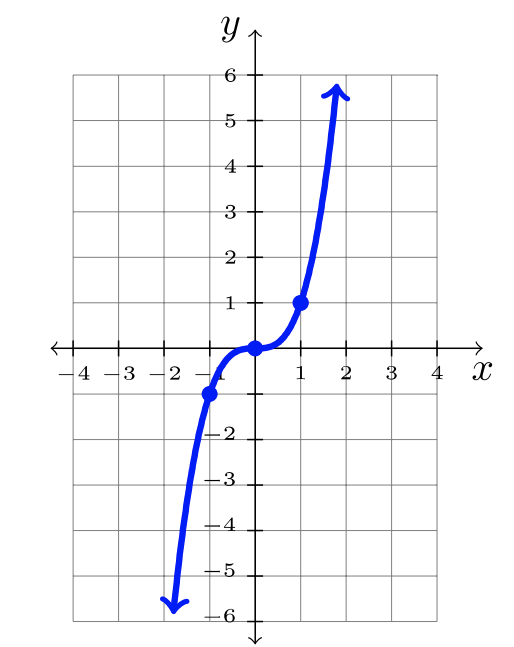
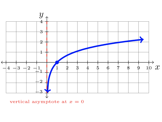
$clipboard_e0ec7b4b76f35f18f5c5d52c9eee803a0.png$	$clipboard_e1f6b7583bfa4bfd9e900f971f6326904.png$	$clipboard_eb5265d3568b1bde6688a1643e83fbb2f.png$

$f(x) = \sqrt{x}$	$f(x) = x^3$	$f(x) = \ln x$
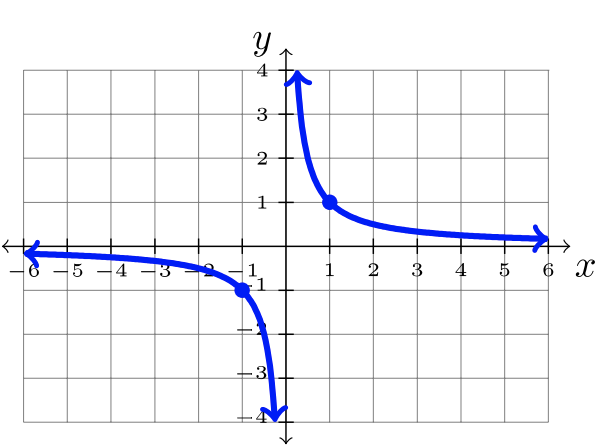
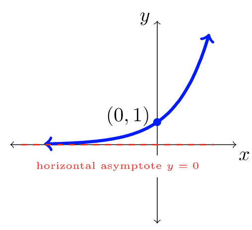
$clipboard_ea79b8b364466de80daf366ac9f77a213.png$	$clipboard_eb696b0dbf8723799beac338367bff4f6.png$	$clipboard_ef55d89ef8d0d94dc91394b9c6ce3e140.png$

$f(x) = \dfrac{1}{x}$	$f(x) = b^x$donde$b>1$	$f(x) = b^x$donde$0 < b< 1$
$clipboard_ee226d5b5690b009e6046c50cb7d2d5c0.png$	$clipboard_e583f09166f4bbaa71c9fd4593537850a.png$	$clipboard_e87fce111b41fff6ce78cf7158cf79a37.png$

Utilizando las transformaciones descritas en la Sección$3.1$, los nueve gráficos mostrados en la página anterior pueden ser desplazados, reflejados, estirados y comprimidos. La comida para llevar para esta sección es reconocer la función padre desde la notación de funciones y aplicar las transformaciones adecuadas para esbozar rápidamente una gráfica o visualizar la gráfica en tu cabeza. ¡Ninguna tecnología es necesaria! Es suficiente tener una comprensión de las funciones y sus gráficas cambiantes.

Ejemplo 3.2.1

Nombra la función padre de la función dada. Luego describa en palabras la (s) transformación (es) en la función padre.

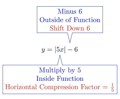
$y = |5x| − 6$
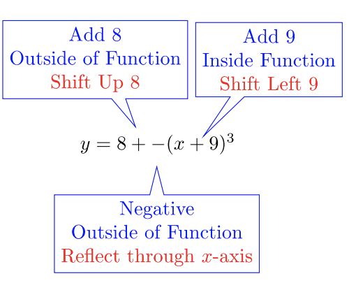
$y = 8 − (x + 9)^3$
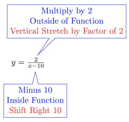
$y = \dfrac{2}{x−10}$

Solución

La función principal es$y = |x|$:

$clipboard_ebfa3193f5b191a25838e1d453b7ad2f1.png$

La función principal es$y = x^3$:

$clipboard_e3e89bc7a9522c97737286bda529f642d.png$

La función principal es$y = \dfrac{1}{x}$:

$clipboard_e4fce349c053cbf533b9a2e3b49ca5f0e.png$

Ejemplo 3.2.2

Utilice la función padre y su (s) transformación (s) para bosquejar la gráfica de la función dada. Es mucho más importante crear un boceto áspero pero preciso sin tecnología que un boceto detallado con tecnología.

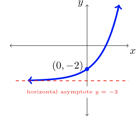
$y = 2^x − 3$
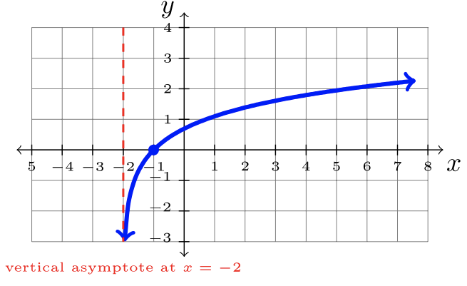
$y = \ln(x + 2)$

Solución

La función padre es$y = b^x$ donde$b = 2 > 1$. Desplazar esta gráfica, incluyendo su asíntota horizontal, hacia abajo$3$ unidades.

$clipboard_e81c6d4d163303c1fc1bd59a171d63ef5.png$

La función padre es$y = \ln x$. Desplazar esta gráfica, incluyendo su asíntota vertical,$2$ unidades izquierdas.

$clipboard_e284658bbaaa0722df9427746025c760b.png$

¡Pruébalo! (Ejercicios)

Para los ejercicios #1 -18, utilice las funciones padre (ver gráficas dentro de esta sección), junto con las transformaciones apropiadas, para crear un boceto de la gráfica de la función dada. No utilice tecnología gráfica.

$y = \dfrac{1}{x+5}$
$y = e^{x−4}$
$y = |x| − 6$
$y = −(x + 2)^3$
$y = 4 + x^2$
$y = \sqrt{x − 4}$
$y = \left( \dfrac{1}{2} \right)^x + 3$
$y = 1 − \sqrt{x}$
$y = |x − 5| + 2$
$y = 1 + (x − 6)^2$
$y = 4 − \dfrac{1}{x}$
$y = 3 + \ln (−x)$
$y = 2\sqrt{x} − 4$
$y = −2(x − 5)^2$
$y = 1 + x^3$
$y = −3|x − 7|$
$y = 5 + \sqrt{-x}$
$y= 3^{x+2} + 4$
Utilice la gráfica de$y = |x|$ y transformaciones para discutir por qué la gráfica de la función transformada$y = |-x|$ es la misma gráfica.
Utilice la gráfica de$y = x^2$ y transformaciones para discutir por qué la gráfica de la función transformada$y = (-x)^2$ es la misma gráfica.
Usando$f(x) = x^2$ como función padre, escribe la función que correspondería a las transformaciones en$f$. No es necesario graficar.

a. Se refleja a través del$x$ eje y las$12$ unidades desplazadas hacia abajo.

b.$10$ Unidades desplazadas hacia la izquierda y$25$ unidades hacia arriba.

Discutir dos enfoques diferentes para transformar la función padre$y = \dfrac{1}{x}$ en gráfica$y = \dfrac{1}{2x}$. ¿Cuáles son las transformaciones? Discutir cómo y por qué cada enfoque producirá la misma gráfica para la nueva función$y = \dfrac{1}{2x}$.

Search

Text Color

Text Size

Margin Size

Font Type

Ejemplo 3.2.1

Ejemplo 3.2.2

\(f(x) = mx + b\)	\(f(x) = x^2\)	\(f(x) = \|x\|\)
$clipboard_e0ec7b4b76f35f18f5c5d52c9eee803a0.png$	$clipboard_e1f6b7583bfa4bfd9e900f971f6326904.png$	$clipboard_eb5265d3568b1bde6688a1643e83fbb2f.png$

\(f(x) = \sqrt{x}\)	\(f(x) = x^3\)	\(f(x) = \ln x\)
$clipboard_ea79b8b364466de80daf366ac9f77a213.png$	$clipboard_eb696b0dbf8723799beac338367bff4f6.png$	$clipboard_ef55d89ef8d0d94dc91394b9c6ce3e140.png$

\(f(x) = \dfrac{1}{x}\)	\(f(x) = b^x\)donde\(b>1\)	\(f(x) = b^x\)donde\(0 < b< 1\)
$clipboard_ee226d5b5690b009e6046c50cb7d2d5c0.png$	$clipboard_e583f09166f4bbaa71c9fd4593537850a.png$	$clipboard_e87fce111b41fff6ce78cf7158cf79a37.png$