
2.4.4E: Ajuste de Modelos Lineales a Datos (Ejercicios)
- Page ID
- 116737

sección 2.4 ejercicio
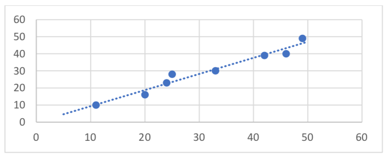
1. A continuación se presentan datos para las puntuaciones del primer y segundo cuestionario para 8 alumnos de una clase. Trace los puntos y luego dibuje una línea que se ajuste a los datos.
| Primer Quiz | 11 | 20 | 24 | 25 | 33 | 42 | 46 | 49 |
| Segundo Quiz | 10 | 16 | 23 | 28 | 30 | 39 | 40 | 49 |
2. Se pidió a ocho estudiantes que estimaran su puntaje en un cuestionario de 10 puntos. Se dan sus puntuaciones estimadas y reales. Trace los puntos y luego dibuje una línea que se ajuste a los datos.
| Predijo | 5 | 7 | 6 | 8 | 10 | 9 | 10 | 7 |
| Real | 6 | 6 | 7 | 8 | 9 | 9 | 10 | 6 |
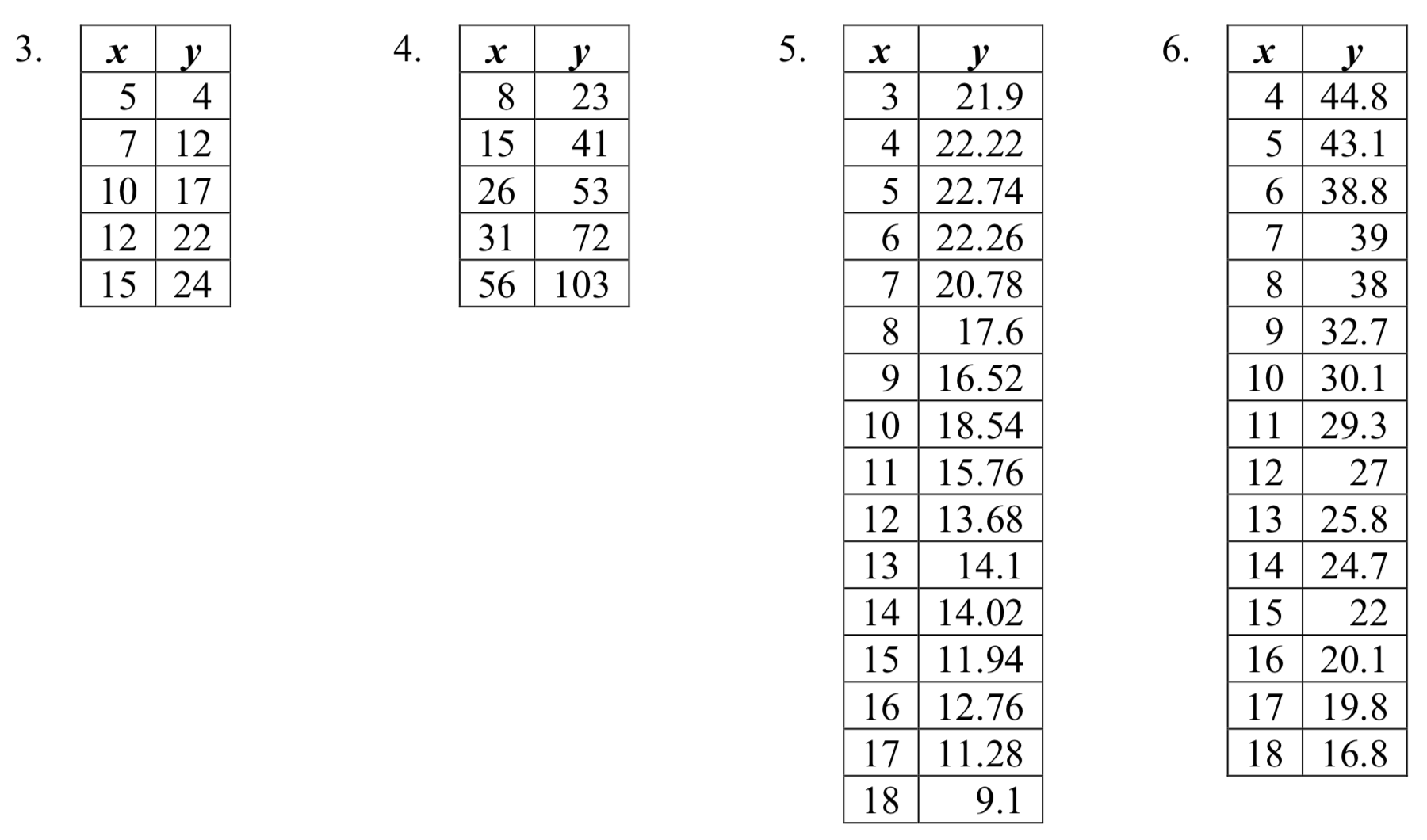
Con base en cada conjunto de datos dados, calcule la línea de regresión usando su calculadora u otra herramienta tecnológica, y determine el coeficiente de correlación.
7. Se realizó una regresión para determinar si existe una relación entre las horas de televisión que se ven al día (\(x\)) y el número de situps que una persona puede hacer (\(y\)). A continuación se dan los resultados de la regresión. Usa esto para predecir la cantidad de situps que puede hacer una persona que ve 11 horas de televisión.
\(y=ax+b\)
\(a=-1.341\)
\(b=32.234\)
\(r^2=0.803\)
\(r=-0.896\)
8. Se realizó una regresión para determinar si existe una relación entre el diámetro de un árbol (\(x\), en pulgadas) y la edad del árbol (\(y\), en años). A continuación se dan los resultados de la regresión. Use esto para predecir la edad de un árbol con diámetro de 10 pulgadas.
\(y=ax+b\)
\(a=6.301\)
\(b=-1.044\)
\(r^2=0.940\)
\(r=0.970\)
Haga coincidir cada diagrama de dispersión que se muestra a continuación con una de las cuatro correlaciones especificadas.
9. \(r = 0.95\)10. \(r = -0.89\)11. \(r = 0.26\)12. \(r = -0.39\)
A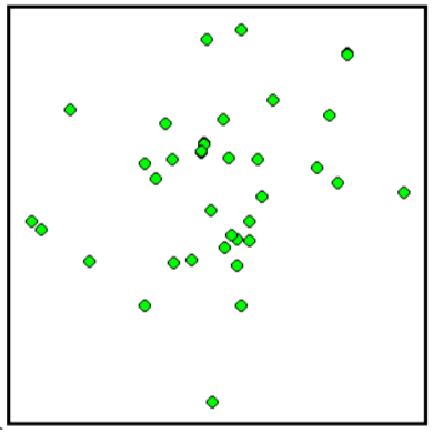 B
B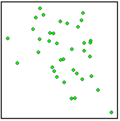 C
C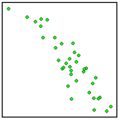 D
D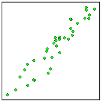
13. El censo de Estados Unidos rastrea el porcentaje de personas de 25 años o más que son egresados universitarios. Esos datos de varios años se dan a continuación. Determinar si la tendencia aparece lineal. Si es así y la tendencia continúa, ¿en qué año el porcentaje superará el 35%?
| Año | 1990 | 1992 | 1994 | 1996 | 1998 | 2000 | 2002 | 2004 | 2006 | 2008 |
| Porcentaje de egresados | 21.3 | 21.4 | 22.2 | 23.6 | 24.4 | 25.6 | 26.7 | 27.7 | 28 | 29.4 |
14. A continuación se da la importación estadounidense de vino (en hectolitros) durante varios años. Determinar si la tendencia aparece lineal. Si es así y la tendencia continúa, ¿en qué año las importaciones superarán los 12 mil hectolitros?
| Año | 1992 | 1994 | 1996 | 1998 | 2000 | 2002 | 2004 | 2006 | 2008 | 2009 |
| Importaciones | 2665 | 2688 | 3565 | 4129 | 4584 | 5655 | 6549 | 7950 | 8487 | 9462 |
- Contestar
-
1.
3. \(y = 1.971x - 3.519\),\(r = 0.967\)
5. \(y = -0.901x + 26.04\),\(r = -0.968\)
7. \(17.483 \approx 17\ situps\)
9. D
11. A
13. Sí, la tendencia aparece lineal porque\(r = 0.994\) y superará el 35% cerca de finales del año 2019.