
4.7.7E: Ajuste de Modelos Exponenciales a Datos (Ejercicios)
- Page ID
- 116817

ejercicio de la sección 4.7
Grafique cada función en una escala semi-logarítmica, luego encuentre una fórmula para la función linealizada en el formulario\(\log \left(f\left(x\right)\right)=mx+b\).
1. \(f\left(x\right)=4\left(1.3\right)^{x}\)
2. \(f\left(x\right)=2\left(1.5\right)^{x}\)
3. \(f\left(x\right)=10\left(0.2\right)^{x}\)
4. \(f\left(x\right)=30\left(0.7\right)^{x}\)
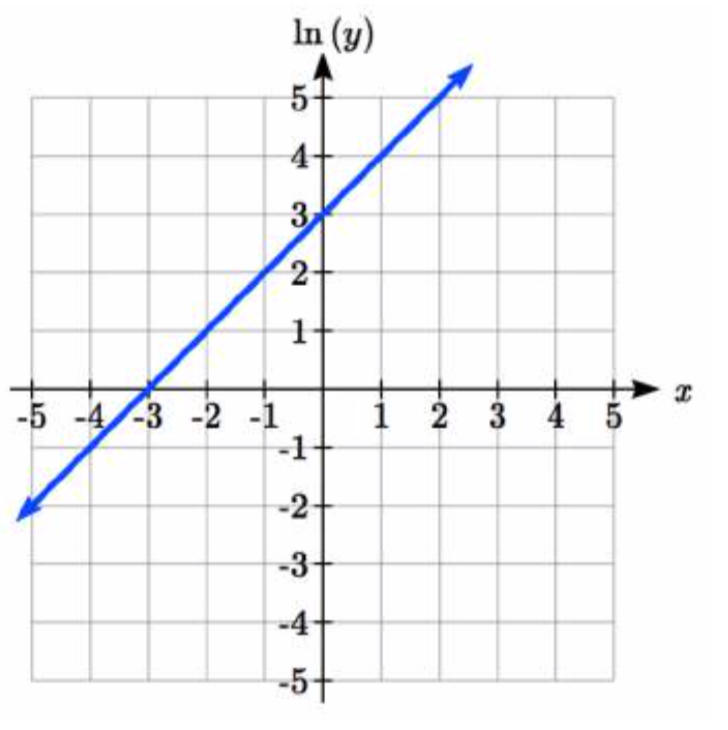
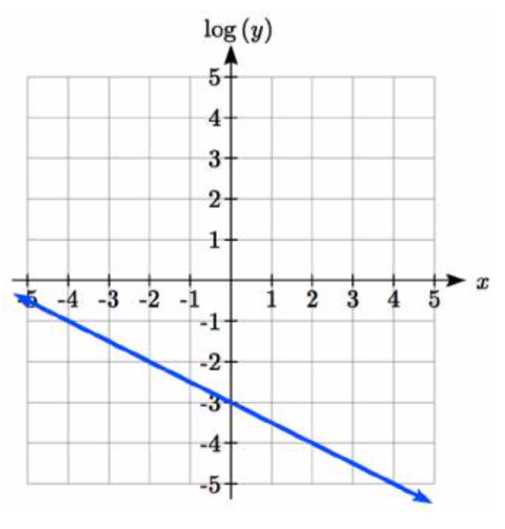
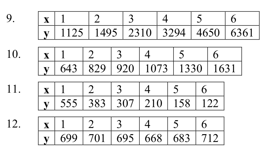
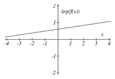
La gráfica a continuación se encuentra en una escala semi-logarítmica, como se indica Encuentra una fórmula para la función exponencial\(y(x)\).
5. 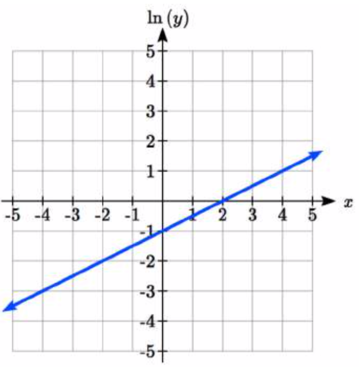 6.
6. 
7. 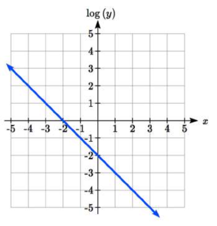 8.
8. 
Utilice la regresión para encontrar una función exponencial que mejor se ajuste a los datos dados.
13. A continuación se muestran los gastos totales (en miles de millones de dólares) en Estados Unidos para la atención en hogares de ancianos. Utilice la regresión para encontrar una función exponencial que modele los datos. ¿Qué predice el modelo que serán los gastos en 2015?
| Año | 1990 | 1995 | 2000 | 2003 | 2005 | 2008 |
| Gasto | 53 | 74 | 95 | 110 | 121 | 138 |
14. La intensidad de la luz a medida que pasa por el agua disminuye exponencialmente con la profundidad. Los datos a continuación muestran la intensidad de la luz (en lúmenes) a diversas profundidades. Utilice la regresión para encontrar una función que modele los datos. ¿Qué predice el modelo que la intensidad será a 25 pies?
| Profundidad (ft) | 3 | 6 | 9 | 12 | 15 | 18 |
| Lumen | 11.5 | 8.6 | 6.7 | 5.2 | 3.8 | 2.9 |
15. A continuación se da el precio promedio de la electricidad (en centavos por kilovatio/hora) de 1990 a 2008. Determinar si un modelo lineal o exponencial se ajusta mejor a los datos, y utilizar el mejor modelo para predecir el precio de la electricidad en 2014.
| Año | 1986 | 1988 | 1990 | 1995 | 1997 | 2000 | 2002 | 2004 | 2006 | 2008 |
| Costo | 7.83 | 8.21 | 8.38 | 8.36 | 8.26 | 8.24 | 8.44 | 8.95 | 10.40 | 11.26 |
16. El costo promedio de una barra de pan blanco de 1986 a 2008 se da a continuación. Determinar si un modelo lineal o exponencial se ajusta mejor a los datos, y usa el mejor modelo para predecir el precio de una barra de pan en 2016.
| Año | 1986 | 1988 | 1990 | 1995 | 1997 | 2000 | 2002 | 2004 | 2006 | 2008 |
| Costo | 0.57 | 0.66 | 0.70 | 0.84 | 0.88 | 0.99 | 1.03 | 0.97 | 1.14 | 1.42 |
- Responder
-
1. \(\text{log} (f(x)) = \text{log} (1.3)x + \text{log} (4)\)
3. \(\text{log} (f(x)) = \text{log} (0.2) x + 1\)
5. \(y = e^{\dfrac{1}{2}x - 1} = e^{-1} e^{\dfrac{1}{2}x} \approx 0.368 (1.6487)^x\)
7. \(y = 10^{-x - 2}. = 10^{-2} 10^{-1x} = 0.01 (0.1)^x\)
9. \(y = 776.682 (1.426)^x\)
11. \(y = 731.92(0.738)^x\)
13. Los gastos son aproximadamente $205
15. \(y = 7.599(1.016)^x\)\(r = 0.83064\),\(y = 0,1493x + 7.4893\),\(r = 0.81713\). Usando la mejor función, predecimos que la electricidad será de 11.157 centavos por kwh