2.3: El desplazamiento vertical de una función trigonométrica
- Page ID
- 117039

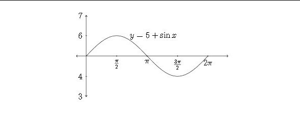
Si se suma o resta una constante a una función trigonométrica, esto afectará a los\(y\) -valores de la función Si consideramos la función\(y-5+\sin x,\) entonces cada uno de los\(y\) valores estándar tendría 5 agregados a if, lo que desplazaría la gráfica hacia arriba 5 unidades.
El siguiente gráfico considera solo los valores cuadránticos para la función sinusoidal:
\ begin {tabular} {|c|c|c|}
\ hline\(\theta\) &\(\sin \theta\) &\(5+\sin \theta\)\\
\ hline 0 & 0 & 5\\
\ hline\(\pi / 2\) & 1 & 6\\ hline
\ hline\(\pi\) & 0 & 5\\
\ hline\(3 \pi / 2\) & -1 & 4\\
\ hline\(2 \pi\) & 0 & 5\\
\ hline
\ end {tabular}
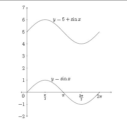
A veces el\(x\) eje -se dibuja a través de la línea que es el nuevo “cero” o “línea media” para la función - en este caso sería\(y-5\)
Al igual que, una constante negativa movería el gráfico hacia abajo, ya que cada valor y sería menor que el\(y\) valor -correspondiente en la función sinusoidal estándar
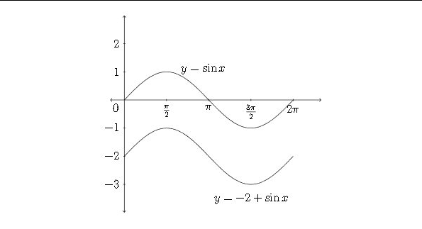
En los ejemplos anteriores la constante se ha escrito frente a la función sinusoidal para mayor claridad. A menudo la constante se escribe después de la función:
\ [\ begin {array} {c}
y-\ sin x+5\
\\ mathrm {or}\\
y-\ sin x-2
\ end {array}
\]
Ahora hemos examinado tres de las cuatro transformaciones de funciones trigonométricas que se discuten en este capítulo: amplitud, periodo y desplazamiento vertical. Una ecuación general para una sinusoide que involucra estas tres transformaciones sería:
\ [
Y=A\ sin (B x) +D
\]
O
\ [
y=A\ cos (B x) +D
\]
Al determinar una ecuación a partir de una gráfica que implica un desplazamiento vertical, el valor de\(A\) will ser la mitad de la distancia entre los valores máximo y mínimo:
\ [
A=\ frac {m a x-m i n} {2}
\]
y el valor de\(D\) será el promedio de los valores máximo y mínimo:
\ [
D=\ frac {m a x+m i n} {2}
\]
Ejemplo
Determinar una ecuación que satisfaga la gráfica dada.
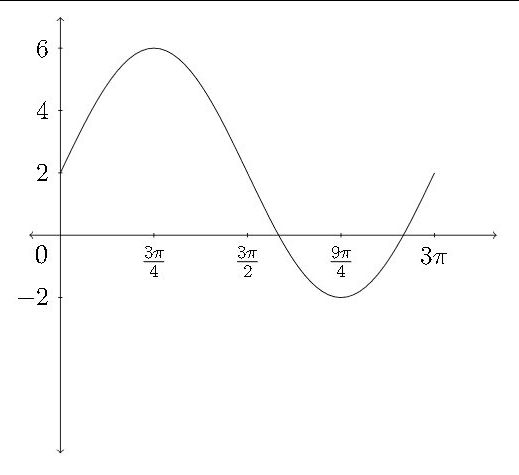
En esta gráfica, el\(y\) valor máximo es 6 y el\(y\) valor mínimo es\(-2 .\) El promedio de estos dos:
\ [
\ frac {m a x+m i n} {2} =\ frac {6+ (-2)} {2} =\ frac {4} {2} =2=D
\]
es el valor del\(D,\) desplazamiento vertical.
La distancia entre 6 y -2 es la\(6-(-2)=8 .\) mitad de la distancia entre el\(\max\) y\(\min\) es\(4,\) que es el valor de\(A\)
\ [\ frac {m a x-m i n} {2} =\ frac {6- (-2)} {2} =\ frac {8} {2} =4=A
\]
La gráfica completa un ciclo completo entre 0 y\(3 \pi,\) así el periodo sería\(3 \pi\) y el valor de\(B\) sería\(B=\frac{2 \pi}{P}=\frac{2 \pi}{3 \pi}=\frac{2}{3}=B .\) Así que una ecuación correcta para la gráfica sería:
\ [
y=4\ sin\ frac {2} {3} x+2
\]
Ejercicios 2.3
Determinar la Amplitud, Período y Desplazamiento Vertical para cada función a continuación y graficar un periodo de la función. Identificar los puntos importantes en los\(y\) ejes\(x\) y.
1. \(\quad y=\sin x+1\)
2. \(\quad y=\cos x-1\)
3. \(\quad y=2 \cos x-\frac{1}{2}\)
4. \(\quad y=5 \sin x+4\)
5. \(\quad y=-\sin \left(\frac{1}{4} x\right)+1\)
6. \(\quad y=-\cos (2 x)+7\)
7. \(\quad y=\frac{1}{3} \sin (\pi x)-4\)
8. \(\quad y=-\frac{1}{2} \cos (2 \pi x)+2\)
9. \(\quad y=5 \cos \left(\frac{1}{2} x\right)+1\)
\(10 . \quad y=4 \sin \left(\frac{1}{3} x\right)-1\)
11. \(\quad y=3 \cos x+2\)
12. \(\quad y=2 \sin x+3\)
13. \(\quad y=2-4 \cos (3 x)\)
14. \(\quad y=5-3 \sin (2 x)\)
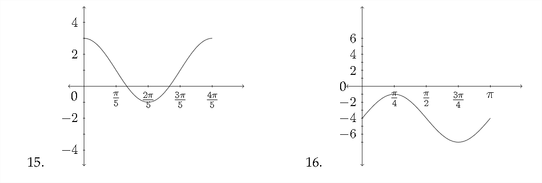
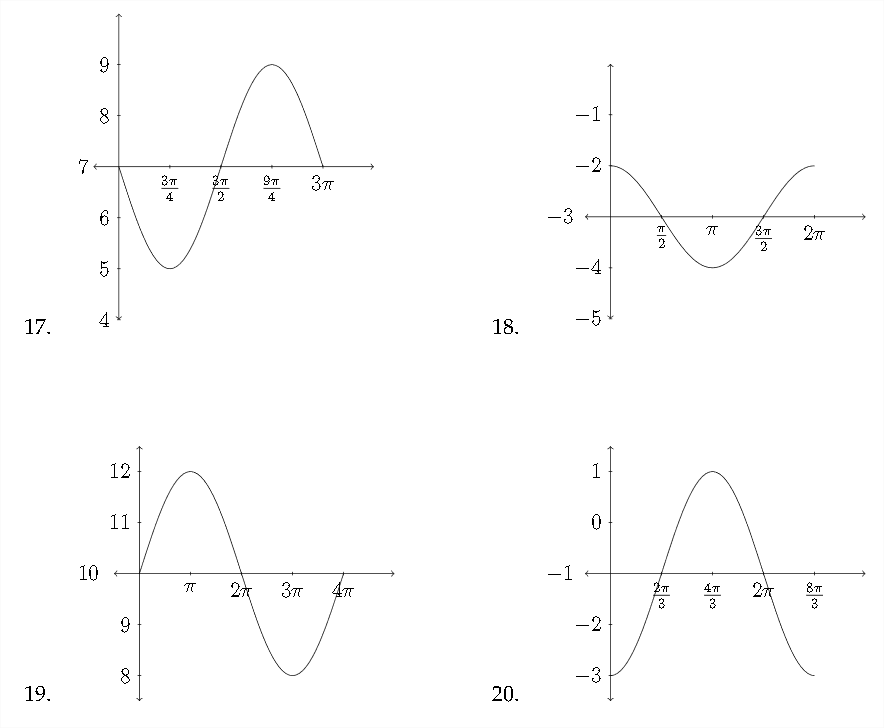
Determinar una ecuación que satisfaga la gráfica dada.