
5.1: Graficar funciones básicas
- Page ID
- 117705

\( \newcommand{\vecs}[1]{\overset { \scriptstyle \rightharpoonup} {\mathbf{#1}} } \)
\( \newcommand{\vecd}[1]{\overset{-\!-\!\rightharpoonup}{\vphantom{a}\smash {#1}}} \)
\( \newcommand{\id}{\mathrm{id}}\) \( \newcommand{\Span}{\mathrm{span}}\)
( \newcommand{\kernel}{\mathrm{null}\,}\) \( \newcommand{\range}{\mathrm{range}\,}\)
\( \newcommand{\RealPart}{\mathrm{Re}}\) \( \newcommand{\ImaginaryPart}{\mathrm{Im}}\)
\( \newcommand{\Argument}{\mathrm{Arg}}\) \( \newcommand{\norm}[1]{\| #1 \|}\)
\( \newcommand{\inner}[2]{\langle #1, #2 \rangle}\)
\( \newcommand{\Span}{\mathrm{span}}\)
\( \newcommand{\id}{\mathrm{id}}\)
\( \newcommand{\Span}{\mathrm{span}}\)
\( \newcommand{\kernel}{\mathrm{null}\,}\)
\( \newcommand{\range}{\mathrm{range}\,}\)
\( \newcommand{\RealPart}{\mathrm{Re}}\)
\( \newcommand{\ImaginaryPart}{\mathrm{Im}}\)
\( \newcommand{\Argument}{\mathrm{Arg}}\)
\( \newcommand{\norm}[1]{\| #1 \|}\)
\( \newcommand{\inner}[2]{\langle #1, #2 \rangle}\)
\( \newcommand{\Span}{\mathrm{span}}\) \( \newcommand{\AA}{\unicode[.8,0]{x212B}}\)
\( \newcommand{\vectorA}[1]{\vec{#1}} % arrow\)
\( \newcommand{\vectorAt}[1]{\vec{\text{#1}}} % arrow\)
\( \newcommand{\vectorB}[1]{\overset { \scriptstyle \rightharpoonup} {\mathbf{#1}} } \)
\( \newcommand{\vectorC}[1]{\textbf{#1}} \)
\( \newcommand{\vectorD}[1]{\overrightarrow{#1}} \)
\( \newcommand{\vectorDt}[1]{\overrightarrow{\text{#1}}} \)
\( \newcommand{\vectE}[1]{\overset{-\!-\!\rightharpoonup}{\vphantom{a}\smash{\mathbf {#1}}}} \)
\( \newcommand{\vecs}[1]{\overset { \scriptstyle \rightharpoonup} {\mathbf{#1}} } \)
\( \newcommand{\vecd}[1]{\overset{-\!-\!\rightharpoonup}{\vphantom{a}\smash {#1}}} \)
Será útil estudiar la forma de las gráficas de algunas funciones básicas, que luego pueden tomarse como bloques de construcción para funciones más avanzadas y complicadas. En esta sección, consideramos las siguientes funciones básicas:
\[y=|x|, \quad y=x^2,\quad y=x^3,\quad y=\sqrt{x},\quad y=\dfrac 1 x \nonumber \]
Podemos graficar estas funciones a mano calculando una tabla, o usando el TI-84, a través de los botones de tabla y gráfico.
- Comenzamos con la función de valor absoluto\(y=|x|\). Recordemos que el valor absoluto se obtiene en la calculadora en el menú matemático pulsando\(\boxed {\text{math}}\boxed {\triangleright } \boxed {\text{enter}}\). El dominio de\(y=|x|\) es todo números reales,\(D=\mathbb{R}\).

Hemos dibujado la gráfica por segunda vez en el\(y\) plano\(x\) - de la derecha.
- De igual manera, obtenemos la gráfica para\(y=x^2\), que es una parábola. El dominio es\(D=\mathbb{R}\).

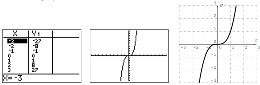
- Aquí está la gráfica para\(y=x^3\). El dominio es\(D=\mathbb{R}\).
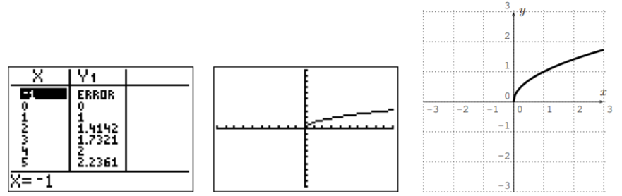
- A continuación graficamos\(y=\sqrt{x}\). El dominio es\(D=[0,\infty)\).
- Por último, aquí está la gráfica para\(y=\dfrac 1 x\). El dominio es\(D=\mathbb{R}-\{0\}\).

Estas gráficas junto con la línea\(y=mx+b\) estudiada en la Sección 2.1 son nuestros bloques de construcción básicos para gráficas más complicadas en las siguientes secciones. Obsérvese en particular, que la gráfica de\(y=x\) es la línea diagonal.
