15.3: Multiplicación Matricial

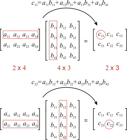
Si\(\mathbf{A}\) tiene dimensiones\(m\times n\) y\(\mathbf{B}\) dimensiones\(n\times p\), entonces el producto\(\mathbf{AB}\) se define, y tiene dimensiones\(m\times p\).

La entrada\((ab)_{ij}\) se obtiene multiplicando fila\(i\) de\(\mathbf{A}\) por columna\(j\) de\(\mathbf{B}\), lo cual se realiza multiplicando las entradas correspondientes juntas y luego sumando los resultados:

Figura\(\PageIndex{1}\): Multiplicación matricial (CC BY-NC-SA; Marcia Levitus)

Ejemplo\(\PageIndex{1}\)

Calcular el producto

\[\begin{pmatrix} 1 &-2 &4 \\ 5 &0 &3 \\ 0 & 1/2 &9 \end{pmatrix}\begin{pmatrix} 1 &0 \\ 5 &3 \\ -1 &0 \end{pmatrix} \nonumber\]

Solución

Necesitamos multiplicar una\(3\times 3\) matriz por una\(3\times 2\) matriz, así que esperamos una\(3\times 2\) matriz como resultado.

\[\begin{pmatrix} 1 &-2 &4 \\ 5 &0 &3 \\ 0 & 1/2 &9 \end{pmatrix}\begin{pmatrix} 1 &0 \\ 5 &3 \\ -1 &0 \end{pmatrix}=\begin{pmatrix} a&b \\ c&d \\ e &f \end{pmatrix} \nonumber\]

Para calcular\(a\), que es entrada (1,1), usamos la fila 1 de la matriz a la izquierda y la columna 1 de la matriz a la derecha:

\[\begin{pmatrix} {\color{red}1} &{\color{red}-2} &{\color{red}4} \\ 5 &0 &3 \\ 0 & 1/2 &9 \end{pmatrix}\begin{pmatrix} {\color{red}1} &0 \\ {\color{red}5} &3 \\ {\color{red}-1} &0 \end{pmatrix}=\begin{pmatrix} {\color{red}a}&b \\ c&d \\ e &f \end{pmatrix}\rightarrow a=1\times 1+(-2)\times 5+4\times (-1)=-13 \nonumber\]

Para calcular\(b\), que es entrada (1,2), usamos la fila 1 de la matriz a la izquierda y la columna 2 de la matriz a la derecha:

\[\begin{pmatrix} {\color{red}1} &{\color{red}-2} &{\color{red}4} \\ 5 &0 &3 \\ 0 & 1/2 &9 \end{pmatrix}\begin{pmatrix} 1&{\color{red}0} \\ 5&{\color{red}3} \\ -1&{\color{red}0} \end{pmatrix}=\begin{pmatrix} a&{\color{red}b} \\ c&d \\ e &f \end{pmatrix}\rightarrow b=1\times 0+(-2)\times 3+4\times 0=-6 \nonumber\]

Para calcular\(c\), que es entrada (2,1), usamos la fila 2 de la matriz a la izquierda y la columna 1 de la matriz a la derecha:

\[\begin{pmatrix} 1&-2&4\\ {\color{red}5} &{\color{red}0} &{\color{red}3} \\ 0 & 1/2 &9 \end{pmatrix}\begin{pmatrix} {\color{red}1} &0 \\ {\color{red}5} &3 \\ {\color{red}-1} &0 \end{pmatrix}=\begin{pmatrix} a&b \\ {\color{red}c}&d \\ e &f \end{pmatrix}\rightarrow c=5\times 1+0\times 5+3\times (-1)=2 \nonumber\]

Para calcular\(d\), que es entrada (2,2), usamos la fila 2 de la matriz a la izquierda y la columna 2 de la matriz a la derecha:

\[\begin{pmatrix} 1&-2&4\\ {\color{red}5} &{\color{red}0} &{\color{red}3} \\ 0 & 1/2 &9 \end{pmatrix}\begin{pmatrix} 1&{\color{red}0} \\ 5&{\color{red}3} \\ -1&{\color{red}0} \end{pmatrix}=\begin{pmatrix} a&b \\ c&{\color{red}d} \\ e &f \end{pmatrix}\rightarrow d=5\times 0+0\times 3+3\times 0=0 \nonumber\]

Para calcular\(e\), que es entrada (3,1), usamos la fila 3 de la matriz a la izquierda y la columna 1 de la matriz a la derecha:

\[\begin{pmatrix} 1&-2&4\\ 5&0&3 \\ {\color{red}0} &{\color{red}1/2} &{\color{red}9} \end{pmatrix}\begin{pmatrix} {\color{red}1} &0 \\ {\color{red}5} &3 \\ {\color{red}-1} &0 \end{pmatrix}=\begin{pmatrix} a&b \\ c&d \\ {\color{red}e} &f \end{pmatrix}\rightarrow e=0\times 1+1/2\times 5+9\times (-1)=-13/2 \nonumber\]

Para calcular\(f\), que es entrada (3,2), usamos la fila 3 de la matriz a la izquierda y la columna 2 de la matriz a la derecha:

\[\begin{pmatrix} 1&-2&4\\ 5&0&3 \\ {\color{red}0} &{\color{red}1/2} &{\color{red}9} \end{pmatrix}\begin{pmatrix} 1&{\color{red}0} \\ 5&{\color{red}3} \\ -1&{\color{red}0} \end{pmatrix}=\begin{pmatrix} a&b \\ c&d \\ e&{\color{red}f} \end{pmatrix}\rightarrow f=0\times 0+1/2\times 3+9\times 0=3/2 \nonumber\]

El resultado es:

\[\displaystyle{\color{Maroon}\begin{pmatrix} 1 &-2 &4 \\ 5 &0 &3 \\ 0 & 1/2 &9 \end{pmatrix}\begin{pmatrix} 1 &0 \\ 5 &3 \\ -1 &0 \end{pmatrix}=\begin{pmatrix} -13&-6 \\ 2&0 \\ -13/2 &3/2 \end{pmatrix}} \nonumber\]

Ejemplo\(\PageIndex{2}\)

Calcular

\[\begin{pmatrix} 1 &-2 &4 \\ 5 &0 &3 \\ \end{pmatrix}\begin{pmatrix} 1 \\ 5 \\ -1 \end{pmatrix}\nonumber\]

Solución

Se nos pide multiplicar una\(2\times 3\) matriz por una\(3\times 1\) matriz (un vector de columna). El resultado será una\(2\times 1\) matriz (un vector).

\[\begin{pmatrix} 1 &-2 &4 \\ 5 &0 &3 \\ \end{pmatrix}\begin{pmatrix} 1 \\ 5 \\ -1 \end{pmatrix}=\begin{pmatrix} a \\ b \end{pmatrix}\nonumber\]

\[a=1\times1+(-2)\times 5+ 4\times (-1)=-13\nonumber\]

\[b=5\times1+0\times 5+ 3\times (-1)=2\nonumber\]

La solución es:

\[\displaystyle{\color{Maroon}\begin{pmatrix} 1 &-2 &4 \\ 5 &0 &3 \\ \end{pmatrix}\begin{pmatrix} 1 \\ 5 \\ -1 \end{pmatrix}=\begin{pmatrix} -13 \\ 2 \end{pmatrix}}\nonumber\]

¿Necesitas ayuda? El siguiente enlace contiene ejemplos resueltos: Multiplicando matrices de diferentes formas (tres ejemplos): http://tinyurl.com/kn8ysqq

Enlaces externos:

• Multiplicando matrices, ejemplo 1: http://patrickjmt.com/matrices-multiplying-a-matrix-by-another-matrix/
• Multiplicando matrices, ejemplo 2: http://patrickjmt.com/multiplying-matrices-example-2/
• Multiplicando matrices, ejemplo 3: http://patrickjmt.com/multiplying-matrices-example-3/

El conmutador

La multiplicación matricial no es, en general, conmutativa. Por ejemplo, podemos realizar

\[\begin{pmatrix} 1 &-2 &4 \\ 5 &0 &3 \\ \end{pmatrix}\begin{pmatrix} 1 \\ 5 \\ -1 \end{pmatrix}=\begin{pmatrix} -13 \\ 2 \end{pmatrix} \nonumber\]

pero no puede realizar

\[\begin{pmatrix} 1 \\ 5 \\ -1 \end{pmatrix}\begin{pmatrix} 1 &-2 &4 \\ 5 &0 &3 \\ \end{pmatrix} \nonumber\]

Incluso con matrices cuadradas, que se pueden multiplicar en ambos sentidos, la multiplicación no es conmutativa. En este caso, es útil definir el conmutador, definido como:

\[[\mathbf{A},\mathbf{B}]=\mathbf{A}\mathbf{B}-\mathbf{B}\mathbf{A} \nonumber\]

Ejemplo\(\PageIndex{3}\)

Dado\(\mathbf{A}=\begin{pmatrix} 3&1 \\ 2&0 \end{pmatrix}\) y\(\mathbf{B}=\begin{pmatrix} 1&0 \\ -1&2 \end{pmatrix}\)

Calcular el conmutador\([\mathbf{A},\mathbf{B}]\)

Solución

\[[\mathbf{A},\mathbf{B}]=\mathbf{A}\mathbf{B}-\mathbf{B}\mathbf{A}\nonumber\]

\[\mathbf{A}\mathbf{B}=\begin{pmatrix} 3&1 \\ 2&0 \end{pmatrix}\begin{pmatrix} 1&0 \\ -1&2 \end{pmatrix}=\begin{pmatrix} 3\times 1+1\times (-1)&3\times 0 +1\times 2 \\ 2\times 1+0\times (-1)&2\times 0+ 0\times 2 \end{pmatrix}=\begin{pmatrix} 2&2 \\ 2&0 \end{pmatrix}\nonumber\]

\[\mathbf{B}\mathbf{A}=\begin{pmatrix} 1&0 \\ -1&2 \end{pmatrix}\begin{pmatrix} 3&1 \\ 2&0 \end{pmatrix}=\begin{pmatrix} 1\times 3+0\times 2&1\times 1 +0\times 0 \\ -1\times 3+2\times 2&-1\times 1+2\times 0 \end{pmatrix}=\begin{pmatrix} 3&1 \\ 1&-1 \end{pmatrix}\nonumber\]

\[[\mathbf{A},\mathbf{B}]=\mathbf{A}\mathbf{B}-\mathbf{B}\mathbf{A}=\begin{pmatrix} 2&2 \\ 2&0 \end{pmatrix}-\begin{pmatrix} 3&1 \\ 1&-1 \end{pmatrix}=\begin{pmatrix} -1&1 \\ 1&1 \end{pmatrix}\nonumber\]

\[\displaystyle{\color{Maroon}[\mathbf{A},\mathbf{B}]=\begin{pmatrix} -1&1 \\ 1&1 \end{pmatrix}}\nonumber\]

Multiplicación de un vector por un escalar

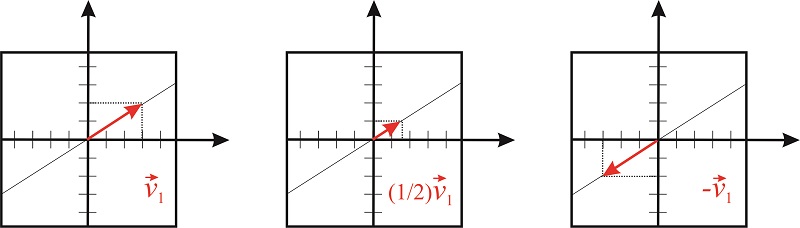
La multiplicación de un vector\(\vec{v_1}\) por un escalar\(n\) produce otro vector de las mismas dimensiones que se encuentra en la misma dirección que\(\vec{v_1}\);

\[n\begin{pmatrix} x \\ y \end{pmatrix}=\begin{pmatrix} nx \\ ny \end{pmatrix} \nonumber\]

El escalar puede estirar o comprimir la longitud del vector, pero no puede girarlo (figure [fig:vector_por_escalar]).

Figura\(\PageIndex{2}\): Multiplicación de un vector por un escalar (CC BY-NC-SA; Marcia Levitus)

Multiplicación de una matriz cuadrada por un vector

La multiplicación de un vector\(\vec{v_1}\) por una matriz cuadrada produce otro vector de las mismas dimensiones de\(\vec{v_1}\). Por ejemplo, podemos multiplicar una\(2\times 2\) matriz y un vector bidimensional:

\[\begin{pmatrix} a&b \\ c&d \end{pmatrix}\begin{pmatrix} x \\ y \end{pmatrix}=\begin{pmatrix} ax+by \\ cx+dy \end{pmatrix} \nonumber\]

Por ejemplo, considere la matriz

\[\mathbf{A}=\begin{pmatrix} -2 &0 \\ 0 &1 \end{pmatrix} \nonumber\]

El producto

\[\begin{pmatrix} -2&0 \\ 0&1 \end{pmatrix}\begin{pmatrix} x \\ y \end{pmatrix} \nonumber\]

es

\[\begin{pmatrix} -2x \\ y \end{pmatrix} \nonumber\]

Vemos que\(2\times 2\) las matrices actúan como operadores que transforman un vector bidimensional en otro vector bidimensional. Esta matriz particular mantiene el valor de\(y\) constante y multiplica el valor de\(x\) por -2 (Figura\(\PageIndex{3}\)).

Figura\(\PageIndex{3}\): Multiplicación de un vector por una matriz cuadrada (CC BY-NC-SA; Marcia Levitus)

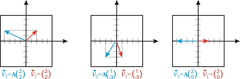
Observe que las matrices son formas útiles de representar operadores que cambian la orientación y el tamaño de un vector. Una clase importante de operadores que son de particular interés para los químicos son los llamados operadores de simetría.