
15.6: Matrices ortogonales
- Page ID
- 70117
Una matriz no singular se llama ortogonal cuando su inverso es igual a su transposición:
\[\mathbf{A}^T =\mathbf{A}^{-1}\rightarrow \mathbf{A}^T\mathbf{A} = \mathbf{I}. \nonumber\]
Por ejemplo, para la matriz
\[\mathbf{A}=\begin{pmatrix} \cos \theta&-\sin \theta \\ \sin \theta&\cos \theta \end{pmatrix}, \nonumber\]
la inversa es
\[ \mathbf{A}^{-1} =\begin{pmatrix} \cos \theta&\sin \theta \\ -\sin \theta&\cos \theta \end{pmatrix} =\mathbf{A}^T \nonumber\]
No necesitamos calcular la inversa para ver si la matriz es ortogonal. Podemos transponer la matriz, multiplicar el resultado por la matriz, y ver si obtenemos la matriz de identidad como resultado:
\[\mathbf{A}^T=\begin{pmatrix} \cos \theta&\sin \theta \\ -\sin \theta&\cos \theta \end{pmatrix} \nonumber\]
\[ \mathbf{A}^T \mathbf{A} =\begin{pmatrix} \cos \theta&\sin \theta \\ -\sin \theta&\cos \theta \end{pmatrix}\begin{pmatrix} \cos \theta&-\sin \theta \\ \sin \theta&\cos \theta \end{pmatrix} =\begin{pmatrix} (\cos^2 \theta+ \sin^2\theta)&0 \\ 0&(\sin^2 \theta+ \cos^2\theta) \end{pmatrix} =\begin{pmatrix} 1&0 \\ 0&1 \end{pmatrix} \nonumber\]
Las columnas de matrices ortogonales forman un sistema de vectores ortonormales (Sección 14.2):
\[\mathbf{M}=\begin{pmatrix} a_1&b_1&c_1 \\ a_2&b_2&c_2 \\ a_3&b_3&c_3 \end{pmatrix}\rightarrow \mathbf{a}=\begin{pmatrix}a_1\\a_2\\a_3\end{pmatrix}; \;\mathbf{b}=\begin{pmatrix}b_1\\b_2\\b_3\end{pmatrix}; \;\mathbf{c}=\begin{pmatrix}c_1\\c_2\\c_3\end{pmatrix} \nonumber\]
\[\mathbf{a}\cdot\mathbf{b}=\mathbf{a}\cdot\mathbf{c}=\mathbf{c}\cdot\mathbf{b}=0 \nonumber\]
\[|\mathbf{a}|=|\mathbf{b}|=|\mathbf{c}|=1 \nonumber\]
Ejemplo\(\PageIndex{1}\)
Demostrar que la matriz\(\mathbf{M}\) es una matriz ortogonal y mostrar que sus columnas forman un conjunto de vectores ortonormales.
\[\mathbf{M}=\begin{pmatrix} 2/3&1/3&-2/3 \\ 2/3&-2/3&1/3 \\ 1/3&2/3&2/3 \end{pmatrix} \nonumber\]
Nota: Este problema también está disponible en formato de video: http://tinyurl.com/k2tkny5
Solución
Primero tenemos que demostrar que\(\mathbf{M}^T\mathbf{M}=1\)
\[\mathbf{M}=\begin{pmatrix} {\color{red}2/3}&{\color{blue}1/3}&-2/3 \\ {\color{red}2/3}&{\color{blue}-2/3}&1/3 \\ {\color{red}1/3}&{\color{blue}2/3}&2/3 \end{pmatrix}\rightarrow \mathbf{M}^T=\begin{pmatrix} {\color{red}2/3}&{\color{red}2/3}&{\color{red}1/3}& \\ {\color{blue}1/3}&{\color{blue}-2/3}&{\color{blue}2/3} \\ -2/3&1/3&2/3 \end{pmatrix} \nonumber\]
\[\mathbf{M}^T\mathbf{M}=\begin{pmatrix} 1&0&0 \\ 0&1&0 \\ 0&0&1 \end{pmatrix}=\mathbf{I} \nonumber\]
Porque\(\mathbf{M}^T\mathbf{M}=\mathbf{I}\), la matriz es ortogonal.
Ahora cómo probar que las columnas para un conjunto de vectores ortonormales. Los vectores son:
\[\mathbf{a}=2/3\mathbf{i}+2/3\mathbf{j}+1/3\mathbf{i}= \begin{pmatrix}2/3\\2/3\\1/3\end{pmatrix}\nonumber\]
\[\mathbf{b}=1/3\mathbf{i}-2/3\mathbf{j}+2/3\mathbf{i}= \begin{pmatrix}1/3\\-2/3\\2/3\end{pmatrix}\nonumber\]
\[\mathbf{c}=-2/3\mathbf{i}+1/3\mathbf{j}+2/3\mathbf{i}= \begin{pmatrix}-2/3\\1/3\\2/3\end{pmatrix}\nonumber\]
Los modulii de estos vectores son:
\[|\mathbf{a}|^2=(2/3)^2+(2/3)^2+(1/3)^2=1 \nonumber\]
\[|\mathbf{b}|^2=(1/3)^2+(-2/3)^2+(2/3)^2=1 \nonumber\]
\[|\mathbf{c}|^2=(-2/3)^2+(1/3)^2+(2/3)^2=1 \nonumber\]
lo que demuestra que los vectores están normalizados.
Los productos de punto de los tres pares de vectores son:
\[\mathbf{a}\cdot\mathbf{b}=(2/3)(1/3)+(2/3)(-2/3)+(1/3)(2/3)=0 \nonumber\]
\[\mathbf{a}\cdot\mathbf{c}=(2/3)(-2/3)+(2/3)(1/3)+(1/3)(2/3)=0 \nonumber\]
\[\mathbf{c}\cdot\mathbf{b}=(-2/3)(1/3)+(1/3)(-2/3)+(2/3)(2/3)=0 \nonumber\]
lo que demuestra que son mutuamente ortogonales.
Debido a que los vectores están normalizados y mutuamente ortogonales, forman un conjunto ortonormal.
Las matrices ortogonales, cuando se consideran operadores que actúan sobre vectores, son importantes porque producen transformaciones que preservan las longitudes de los vectores y los ángulos relativos entre ellos. Por ejemplo, en dos dimensiones, la matriz
\[\mathbf{M}_1=1/\sqrt{2}\begin{pmatrix} 1&1 \\ 1&-1 \end{pmatrix} \nonumber\]
es un operador que gira un vector\(\pi/4\) en sentido contrario a las agujas del reloj (Figura\(\PageIndex{1}\)) preservando las longitudes de los vectores y su orientación relativa. En otras palabras, una matriz ortogonal gira una forma sin distorsionarla. Si las columnas son vectores ortogonales que no están normalizados, como en
\[\mathbf{M}_2=\begin{pmatrix} 1&1 \\ 1&-1 \end{pmatrix}, \nonumber\]
el objeto cambia de tamaño pero la forma no se distorsiona. Sin embargo, si las dos columnas son vectores no ortogonales, la transformación distorsionará la forma. La figura\(\PageIndex{1}\) muestra un ejemplo con la matriz
\[\mathbf{M}_3=\begin{pmatrix} 1&2 \\ -1&1 \end{pmatrix} \nonumber\]
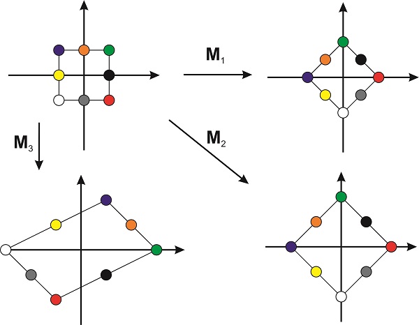
De esta discusión, no debería sorprenderle que todas las matrices que representan operadores de simetría (Sección 15.4) sean matrices ortogonales. Estos operadores se utilizan para rotar y reflejar el objeto alrededor de diferentes ejes y planos sin distorsionar su tamaño y forma.