1.15: Reducción de representaciones II

Al aprovechar al máximo la simetría molecular, a menudo simplificamos enormemente los problemas relacionados con las propiedades moleculares. Por ejemplo, la formación de enlaces químicos depende fuertemente de que los orbitales atómicos involucrados tengan las simetrías correctas. Para hacer pleno uso de la teoría de grupos en las aplicaciones que estaremos considerando, necesitamos desarrollar un poco más de 'maquinaria'. Específicamente, dado un conjunto de bases (de orbitales atómicos, por ejemplo) necesitamos averiguar:

1. Cómo determinar las representaciones irreducibles abarcadas por las funciones base
2. Cómo construir combinaciones lineales de las funciones básicas originales que se transforman como una especie de representación/simetría irreducible dada.

Resulta que ambos problemas se pueden resolver usando algo llamado el 'Gran Teorema de Ortogonalidad' (GOT para abreviar). El GOT resume una serie de relaciones de ortogonalidad implícitas en representaciones matriciales de grupos de simetría, y pueden derivarse de una manera algo cualitativa considerando estas relaciones a su vez.

A algunos de ustedes les puede resultar un poco difícil la siguiente sección. En ella, derivaremos dos expresiones importantes que podremos utilizar para lograr los dos objetivos que hemos expuesto anteriormente. No es importante que entiendas cada paso en estas derivaciones; principalmente se han incluido solo para que puedas ver de dónde vienen las ecuaciones. Sin embargo, necesitarás entender cómo usar los resultados. Esperemos que esto no le resulte demasiado difícil una vez que hayamos trabajado a través de algunos ejemplos.

Conceptos generales de ortogonalidad

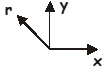
Probablemente ya estés familiarizado con el concepto geométrico de ortogonalidad. Dos vectores son ortogonales si su producto de punto (es decir, la proyección de un vector sobre el otro) es cero. Un ejemplo de un par de vectores ortogonales es proporcionado por\(\textbf{x}\) and \(\textbf{y}\) Cartesian unit vectors.

\[\textbf{x}, \textbf{y} = 0\label{15.1}\]

Una consecuencia de la ortogonalidad de\(\textbf{x}\) and \(\textbf{y}\) is that any general vector in the \(xy\) plane may be written as a linear combination of these two basis vectors.

\[\textbf{r} = a\textbf{x} + b\textbf{y} \label{15.2}\]

Las funciones matemáticas también pueden ser ortogonales. Dos funciones,\(f_1(x)\) and \(f_2(x)\), are defined to be orthogonal if the integral over their product is equal to zero i.e.

\[\int f_1(x) f_2(x) dx = \delta_{12}\]

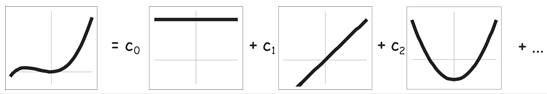
Esto simplemente significa que debe haber 'no superposición' entre las funciones ortogonales, que es lo mismo que el requisito de ortogonalidad para los vectores, arriba. De la misma manera que para los vectores, cualquier función general puede escribirse como una combinación lineal de un conjunto adecuadamente elegido de funciones de base ortogonales. Por ejemplo, los polinomios de Legendre\(P_n(x)\) form an orthogonal basis set for functions of one variable \(x\).

\[f(x) = \sum_n c_n P_n(x) \label{15.3}\]

Relaciones de ortogonalidad en la Teoría de Grupos

Las representaciones irreducibles de un grupo de puntos satisfacen una serie de relaciones de ortogonalidad:

1. Si los elementos correspondientes de la matriz en todos los representantes de la matriz de una representación irreducible se cuadran y se suman, el resultado es igual al orden del grupo dividido por la dimensionalidad de la representación irreducible. i.e.

\[\sum _g \Gamma_k(g)_{ij} \Gamma_k(g)_{ij} = \dfrac{h}{d_k} \label{15.4}\]

donde\(k\) labels the irreducible representation, \(i\) and \(j\) label the row and column position within the irreducible representation, \(h\) is the order of the group, y\(d_k\) is the order of the irreducible representation. e.g. The order of the group \(C_{3v}\) is 6. If we apply the above operation to the first element in the 2x2 (\(E\)) irreducible representation derivado en la Sección 12, el resultado debe ser igual a\(\dfrac{h}{d_k}\) = \(\dfrac{6}{2}\) = 3. Carrying out this operation gives:

\[(1)^2 + (-\dfrac{1}{2})^2 + (-\dfrac{1}{2})^2 + (1)^2 + (-\dfrac{1}{2})^2 +(-\dfrac{1}{2})^2 = 1 + \dfrac{1}{4} + \dfrac{1}{4} + 1 + \dfrac{1}{4} + \dfrac{1}{4} = 3 \label{15.5}\]

2. Si en lugar de sumar los cuadrados de los elementos de la matriz en una representación irreducible, sumamos el producto de dos elementos diferentes de dentro de cada matriz, el resultado es igual a cero. i.e.

\[\sum _g \Gamma_k(g)_{ij} \Gamma_k(g)_{i'j'} = 0 \label{15.6}\]

donde\(i \neq i'\) y/o\(j \neq j'\) . Por ejemplo, si realizamos esta operación usando los dos elementos de la primera fila de la representación irreducible 2D utilizada en 1, obtenemos:

\[(1)(0) + (-\dfrac{1}{2})(\dfrac{\sqrt{3}}{2}) + (-\dfrac{1}{2})(-\dfrac{\sqrt{3}}{2}) + (1)(0) + (-\dfrac{1}{2})(\dfrac{\sqrt{3}}{2}) + (-\dfrac{1}{2})(-\dfrac{\sqrt{3}}{2}) = 0 + \dfrac{\sqrt{3}}{4} - \dfrac{\sqrt{3}}{4} + 0 - \dfrac{\sqrt{3}}{4} + \dfrac{\sqrt{3}}{4} = 0 \label{15.7}\]

3. Si sumamos el producto de dos elementos a partir de las matrices de dos representaciones irreducibles diferentes\(k\) and \(m\), the result is equal to zero. i.e.

\[\sum_g \Gamma_k(g)_{ij} \Gamma_m(g)_{i'j'} = 0 \label{15.8}\]

donde ahora no hay restricción en los valores de los índices\(i\), \(i'\), \(j\), \(j'\) (apart from the rather obvious restriction that they must be less than or equal to the dimensions of the irreducible representation). por ejemplo Realizar esta operación en los primeros elementos de la\(A_1\) and \(E\) irreducible representations we derived for \(C_{3v}\) gives:

\[(1)(1) + (1)(-\dfrac{1}{2}) + (1)(-\dfrac{1}{2}) + (1)(1) + (1)(-\dfrac{1}{2}) + (1)(-\dfrac{1}{2}) = 1 - \dfrac{1}{2} - \dfrac{1}{2} + 1 - \dfrac{1}{2} - \dfrac{1}{2} = 0 \label{15.9}\]

Podemos combinar estos tres resultados en una ecuación general, el Teorema de la Gran Ortogonalidad\(^4\).

\[\sum_g \Gamma_k(g)_{ij} \Gamma_m(g)_{i'j'} = \dfrac{h}{\sqrt{d_kd_m}} \delta_{km} \delta_{ii'} \delta_{jj'} \label{15.10}\]

Para la mayoría de las aplicaciones en realidad no necesitamos el Teorema completo de la Gran Ortogonalidad. Un poco de artimaña matemática transforma Ecuación\(\ref{15.10}\) into the ‘Little Orthogonality Theorem’ (or LOT), which is expressed in terms of the characters of the irreducible representations rather than the irreducible representations themselves.

\[\sum_g \chi_k(g) \chi_m(g) = h\delta_{km} \label{15.11}\]

Dado que los caracteres para dos operaciones de simetría en la misma clase son los mismos, también podemos reescribir las operaciones de suma sobre simetría como una suma sobre clases.

\[\sum_C n_C \chi_k(C) \chi_m(C) = h \delta_{km} \label{15.12}\]

donde\(n_C\) is the number of symmetry operations in class \(C\).

En todos los ejemplos que hemos considerado hasta ahora, los personajes han sido reales. Sin embargo, esto no es necesariamente cierto para todos los grupos de puntos, por lo que para que las ecuaciones anteriores sean completamente generales necesitamos incluir la posibilidad de caracteres imaginarios. En este caso tenemos:

\[\sum_C n_C \chi_k^*(C) \chi_m(C) = h \delta_{km} \label{15.13}\]

donde\(\chi_k^*(C)\) está el complejo conjugado de\(\chi_k(C)\). Ecuación\(\ref{15.13}\) is of course identical to Equation \(\ref{15.12}\) when all the characters are real.

Uso del LOT para determinar las representaciones irreducibles abarcadas por una base

En la Sección\(12\) we discovered that we can often carry out a similarity transform on a general matrix representation so that all the representatives end up in the same block diagonal form. When this is possible, each set of submatrices also forms a valid matrix representation of the group. If none of the submatrices can be reduced further by carrying out another similarity transform, they are said to form an irreducible representation of the point group. An important property of matrix representatives is that their character is invariant under a similarity transform. This means that the character of the original representatives must be equal to the sum of the characters of the irreducible representations into which the representation is reduced. e.g. if we consider the representative for the \(C_3^-\) symmetry operation in our \(NH_3\) example, we have:

\[\begin{array}{ccccc} \begin{pmatrix} 1 & 0 & 0 & 0 \\ 0 & 0 & 0 & 1 \\ 0 & 1 & 0 & 0 \\ 0 & 0 & 1 & 0 \end{pmatrix} & \begin{array}{c} \text{similarity transform} \\ \longrightarrow \end{array} & \begin{pmatrix} 1 & 0 & 0 & 0 \\ 0 & 1 & 0 & 0 \\ 0 & 0 & -\dfrac{1}{2} & -\dfrac{\sqrt{3}}{2} \\ 0 & 0 & \dfrac{\sqrt{3}}{2} & -\dfrac{1}{2} \end{pmatrix} & = & (1) \otimes (1) \otimes \begin{pmatrix} -\dfrac{1}{2} -\dfrac{\sqrt{3}}{2} \\ \dfrac{\sqrt{3}}{2} -\dfrac{1}{2} \end{pmatrix} \\ \chi = 1 & & \chi = 1 & & \chi = 1 + 1 - 1 = 1 \end{array} \label{15.14}\]

De ello se deduce que podemos escribir los caracteres para una representación general\(\Gamma(g)\) en términos de los caracteres de las representaciones irreducibles\(\Gamma_k(g)\) en las que se puede reducir.

\[\chi(g) = \sum_k a_k \chi_k(g) \label{15.15}\]

donde los coeficientes\(a_k\) in the sum are the number of times each irreducible representation appears in the representation. This means that in order to determine the irreducible representations spanned by a given basis. all we have to do is determine the coefficients \(a_k\) in the above equation. This is where the Little Orthogonality Theorem comes in handy. If we take el LOT en forma de Ecuación\(\ref{15.15}\), and multiply each side through by \(a_k\), we get

\[\Sigma_g a_k \chi_k(g) \chi_m(g) = h a_k \delta_{km} \label{15.16}\]

Sumando ambos lados de la ecuación anterior\(k\) gives

\[\Sigma_g \Sigma_k a_k \chi_k(g) \chi_m(g) = h \Sigma_k a_k \delta_{km} \label{15.17}\]

Podemos usar\(\ref{15.15}\) to simplify the left hand side of this equation. Also, the sum on the right hand side reduces to \(a_m\) because \(\delta{km}\) La ecuación es solo distinta de cero (e igual a\(1\)) when \(k\) = \(m\)

\[\Sigma_g \chi(g) \chi_m(g) = h a_m \label{15.18}\]

Dividiendo ambos lados por\(h\) (the order of the group), gives us an expression for the coefficients \(a_m\) in terms of the characters \(\chi(g)\) de la representación original y los personajes\(\chi_m(g)\) del\(m^{th}\) irreducible representation.

\[ a_m = \dfrac{1}{h} \Sigma_g \chi(g) \chi_m(g) \label{15.19}\]

Por supuesto, podemos escribir esto como una suma sobre clases en lugar de una suma sobre operaciones de simetría.

\[a_m = \dfrac{1}{h} \Sigma_C n_C \chi(g) \chi_m(g) \label{15.20}\]

Como ejemplo, en la Sección\(12\) we showed that the matrix representatives we derived for the \(C_{3v}\) group could be reduced into two irreducible representations of \(A_1\) symmetry and one of \(E\) symmetry. i.e. \(\Gamma\) = 2\(A_1\) + \(E\). We could have obtained the same result using Equation \(\ref{15.20}\)). The characters for our original representation and for the irreducible representations of the \(C_{3v}\) point group (\(A_1\), \(A_2\) and \(E\)) are given in the table below.

\[\begin{array}{llll} \hline C_{3v} & E & 2C_3 & 3\sigma_v \\ \hline \chi & 4 & 1 & 2 \\ \hline \chi(A_1) & 1 & 1 & 1 \\ \chi(A_2) & 1 & 1 & -1 \\ \chi(E) & 2 & -1 & 0 \\ \hline \end{array} \label{15.21}\]

De Ecuación\(\ref{15.20}\), the number of times each irreducible representation occurs for our chosen basis \(\begin{pmatrix} s_n, s_1, s_2, s_3 \end{pmatrix}\) is therefore

\[\begin{array}{l} a(A_1) = \dfrac{1}{6}(1x4x1 + 2x1x1 + 3x2x1) = 2 \\ a(A_2) = \dfrac{1}{6}(1x4x1 + 2x1x1 + 3x2x-1) = 0 \\ a(E) = \dfrac{1}{6}(1x4x2 + 2x1x-1 + 3x2x0) = 1 \end{array} \label{15.22}\]

es decir, nuestra base se extiende por\(2A_1\) + \(E\), as we found before.

---

\(^4\)The \(\delta_{ij}\)apareciendo en Ecuación\(\ref{15.10}\) are called Dirac delta functions. They are equal to \(1\) if \(i\) = \(j\) and \(0\) otherwise.